작성자 : 이재빈

Contents

0. Intro
1. Deep Learning for Graphs
2. Graph Convolutional Network
3. Graph Attention Network
4. Application

Keyword : Deep Learning on Graph , Neighborhood Aggregation , GNN , GCN , GAT

0. Intro

Node Embedding

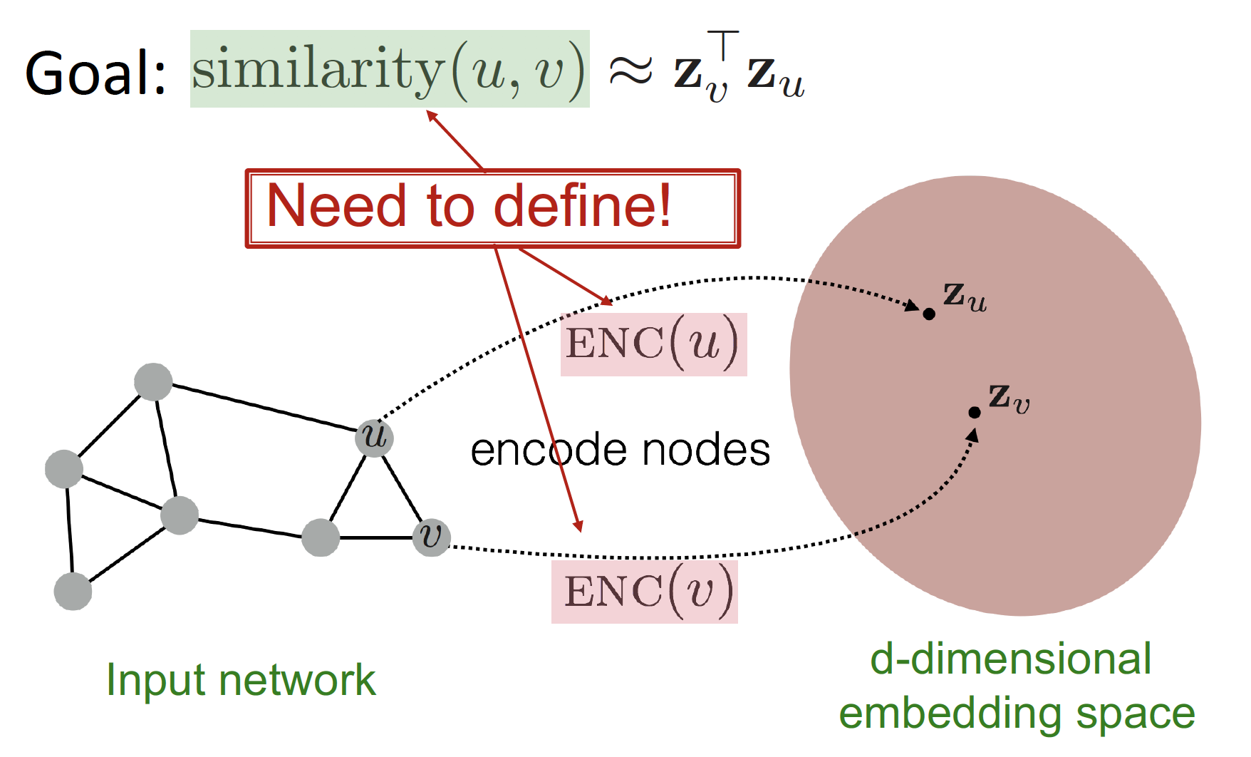
7강에서는 Node Embedding 에 대해 공부했습니다.
embedding node ($z_u$, $z_v$) 사이의 관계가 original network node ($u$, $v$) 사이의 관계 (Similarity) 를 가장 잘 표현해 주는 encoder ($ENC(⋅)$) 를 찾는 방법을 배웠습니다.

From "Shallow" to "Deep"

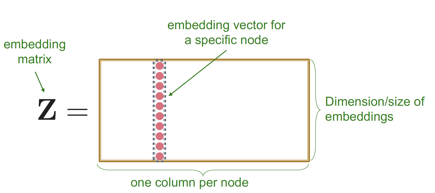
이 때 Shallow Encoder (Lookup table) 를 공부했습니다.
Shallow Encoder는 single layer ($f$) 로 구성되어 있으며, 이를 통해 node embedding 을 진행하고 ($u$ → $z_u$), similarity (${z_v}^T z_u$) 를 계산합니다.

Limitations of Shallow Embedding

1. $O(|V|)$ parameters are needed
   • parameter 개수 = # of nodes
     node 끼리 parameter 를 공유하지 않습니다.
   • 각 node 들은 unique embedding 값을 가지게 됩니다.
2. Inherently "transductive"
   • I have to re-embed everything
   • train 과정에서 보지 않은 node/embedding 을 generalize 할 수 없습니다.
3. Do not incorporate node features
   • node attribute feature 를 사용하지 않습니다.

---

Deep Graph Encoders

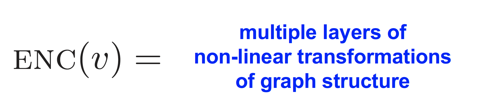
따라서 위의 한계를 극복하고자, multiple layer 로 구성된 Deep Encoder 를 고려하게 됩니다.

Challenges

Graph Network 를 Deep Neural Network 구조에 통과시켜서, node embedding (good prediction) 을 만들어 내고 싶지만, 이는 쉽지 않습니다.

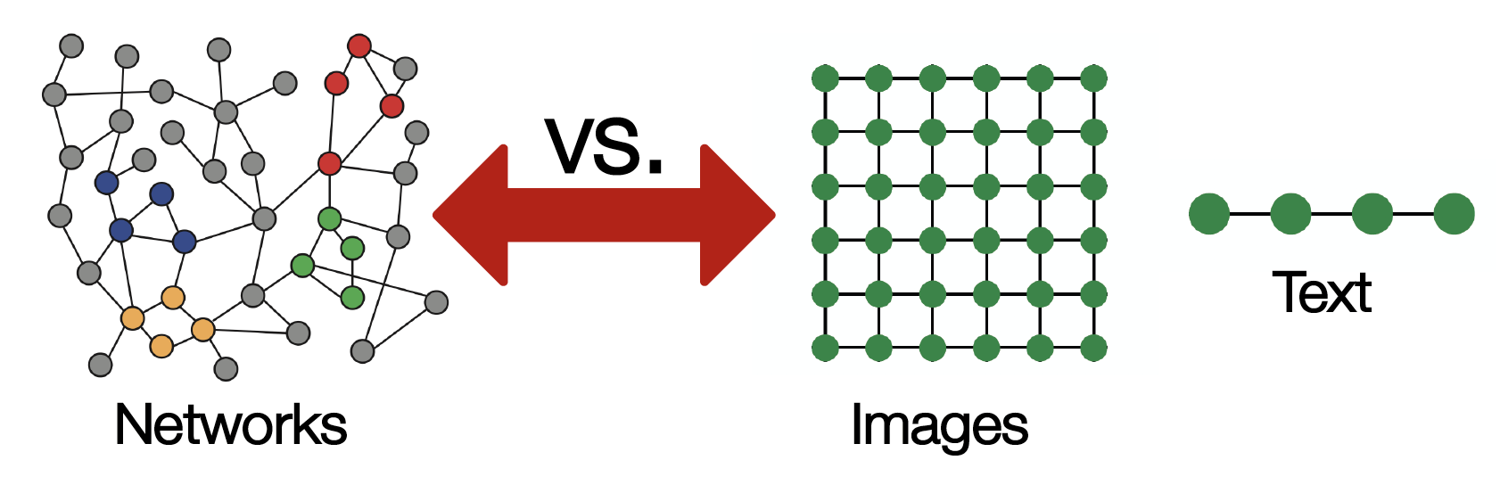
단순하게 Deep Learning을 적용하기에는, 실제 Network가 매우 복잡하기 때문입니다.

• 현존하는 ML/DL ToolBox 는 Image (Grids = Fixed Size Graph) & Text (Sequences = Line Graph) 에 특화되어 있습니다.
• Network는 위상학적으로 매우 복잡한 구조를 가지고 있습니다.
• node들은 고정된 순서 & 기준점이 없습니다.
• dynamic 하며, Multimodal features를 갖는 경우도 있습니다.

A Naive Approach

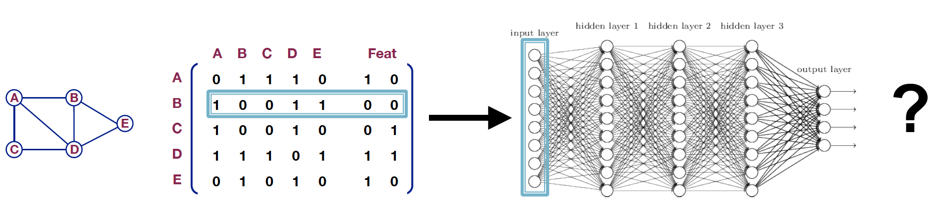
Adjacency matrix 와 Feature vector 를 concat 해서 Deep Neural Network 의 input 으로 넣는 방법 또한 적용이 어렵습니다.

Issues

1. $O(N)$ : parameter 개수 (node + feature) 가 많아집니다.
2. different size 의 graph 에 적용할 수 없습니다.
3. node 의 순서가 바뀌면, 의미가 달라질 수 있습니다.
   • Adj node 의 ordering 이 shuffle 될 수도 있습니다.
   • 2 additional feature node 를 어디에 넣어야 할지 모호해집니다.

idea : Convolutional Networks

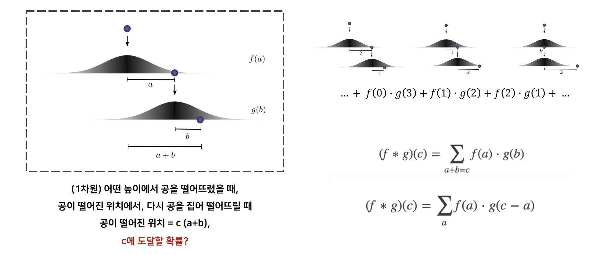
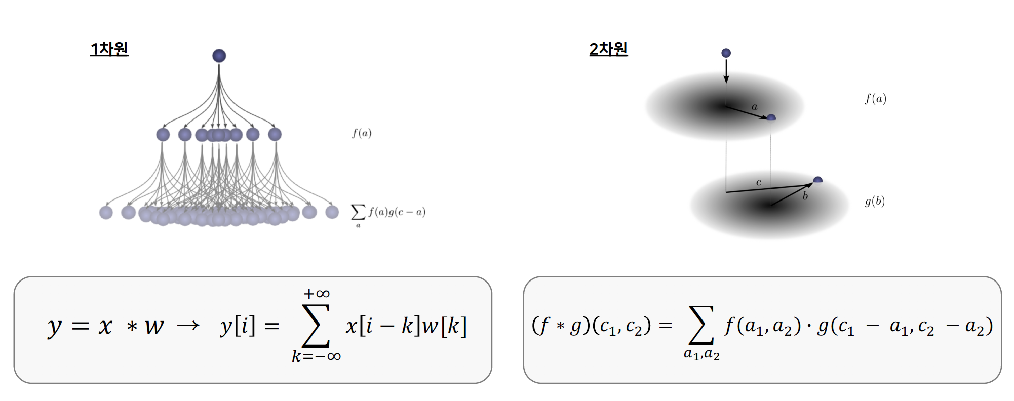
Convolutional 연산의 원리는 위와 같습니다.
sliding window 통해 얻은 정보를 다 더하여, output 을 도출합니다.

$(f \ast g)(t) = \int_{a}^{b} f(\tau) g(t-\tau) \, d\tau$

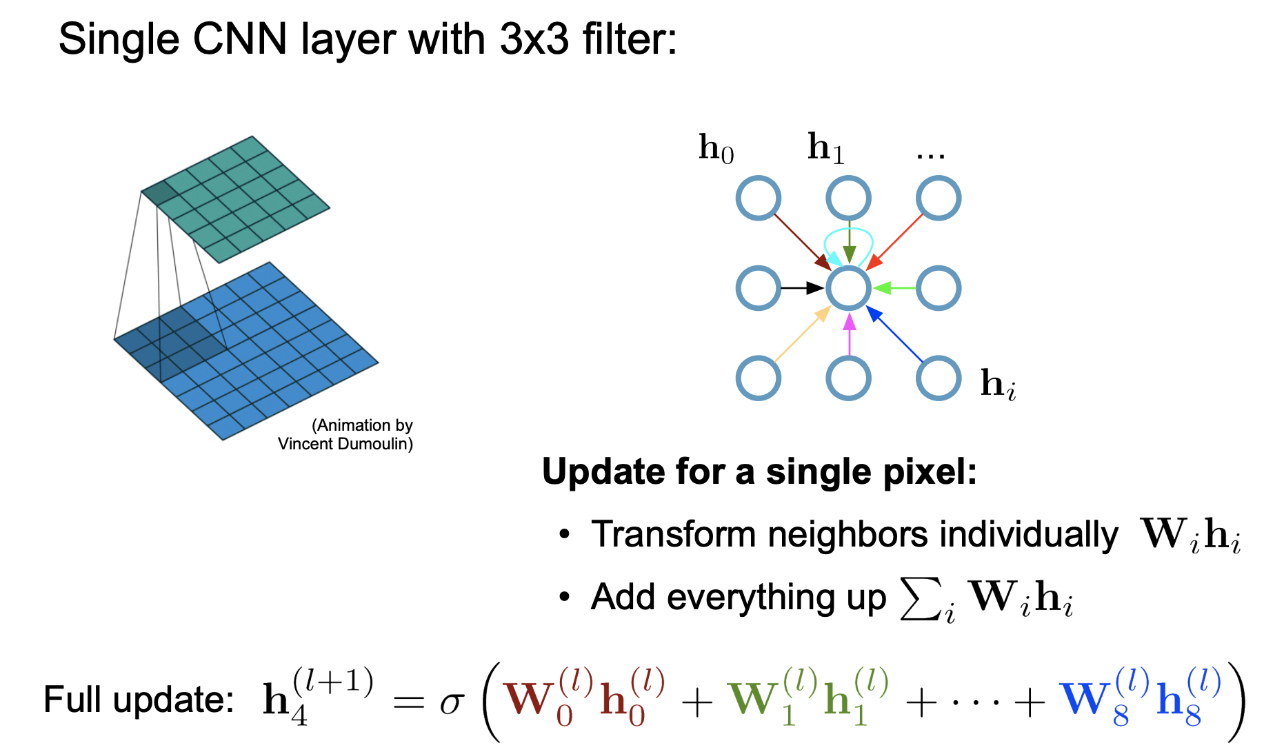
neighborhood 의 message 를 collect 하여, node 의 message 와 combine 하고, 이를 통해 new value 를 produce 하고자 합니다.

이러한 과정을 가장 잘 수행할 수 있는 연산 방법이 ConV 이기 때문에,
Convolutional 을 graph 에 적용해서, information 을 aggregate 하고자 합니다.

1. Deep Learning for Graphs

Setup

graph $G$ 에 대하여,

• $V$ : vertex set = node 집합
• $A$ : Adjacency matrix = 인접행렬
• $X$ : Node Feature matrix

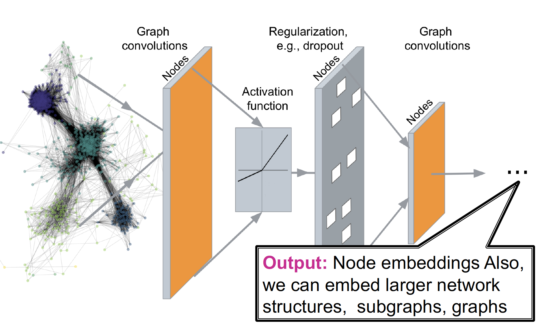
Graph Convolutional Networks

Learn how to propagate information across the graph to compute node features

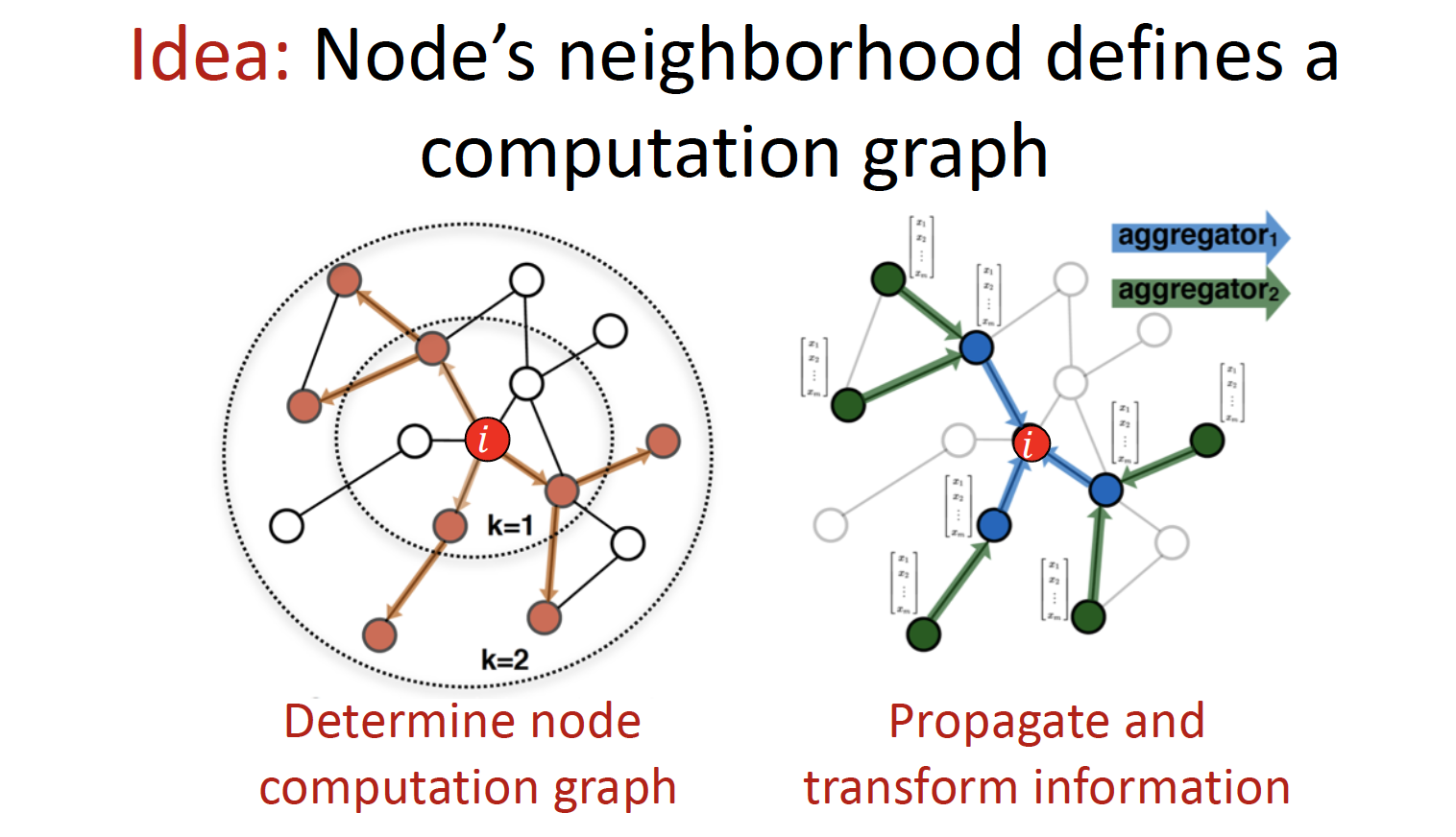
node i 에 대한 prediction 을 하고 싶을 때,
1. node computation graph 를 결정하고,
2. neighborhood information 을 propagate 하고 aggregate 합니다.

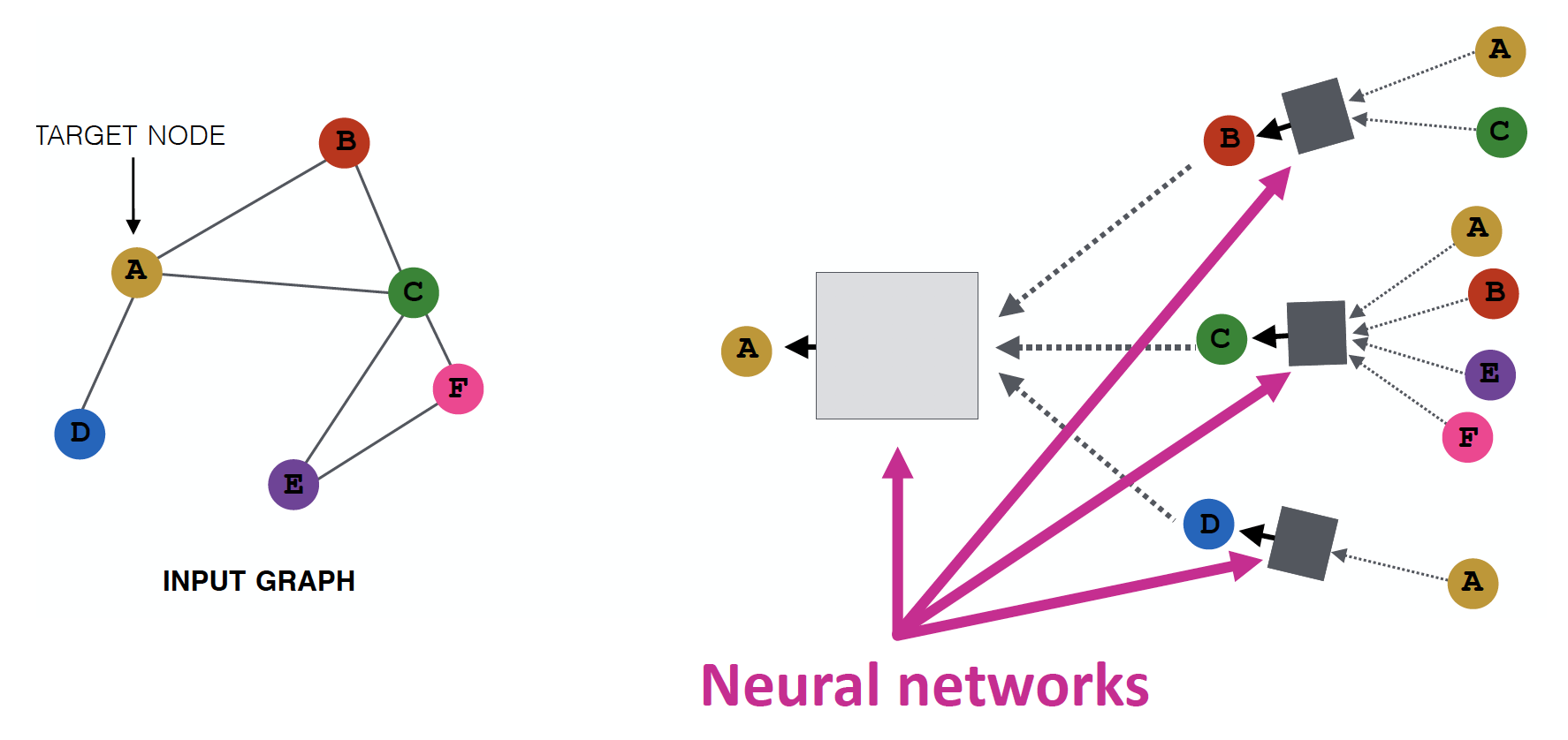
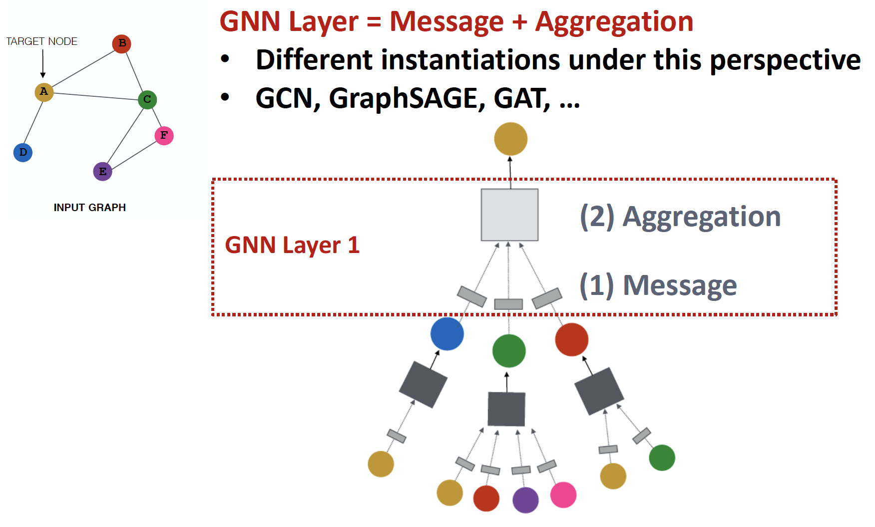
Aggregate Neighbors

Key idea

Local Network Neighborhoods 정보를 기반으로 node embedding 을 진행합니다.

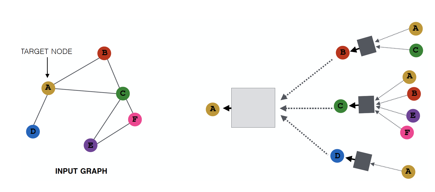
• node B 는 A, C 로 부터, node A 는 B, C, D 로 부터 정보를 얻습니다.
• Graph 에서는 4~5 level 이상의 Layer를 쌓지 않는데, (Ch2 MSN 예시에서도 path length = 6.6 이었듯이) Depth 6 정도면 graph 내의 모든 node 를 방문할 수 있기 때문입니다.

Intuition 1

Neural Network 를 통해 neighborhood information 을 aggregate 합니다.

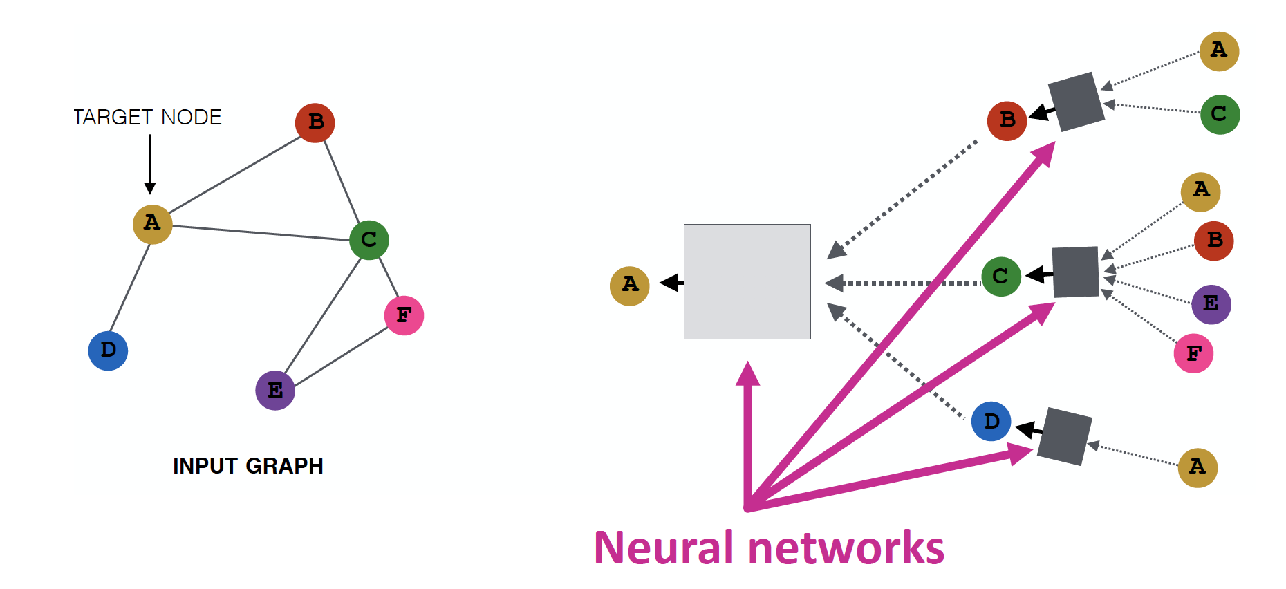
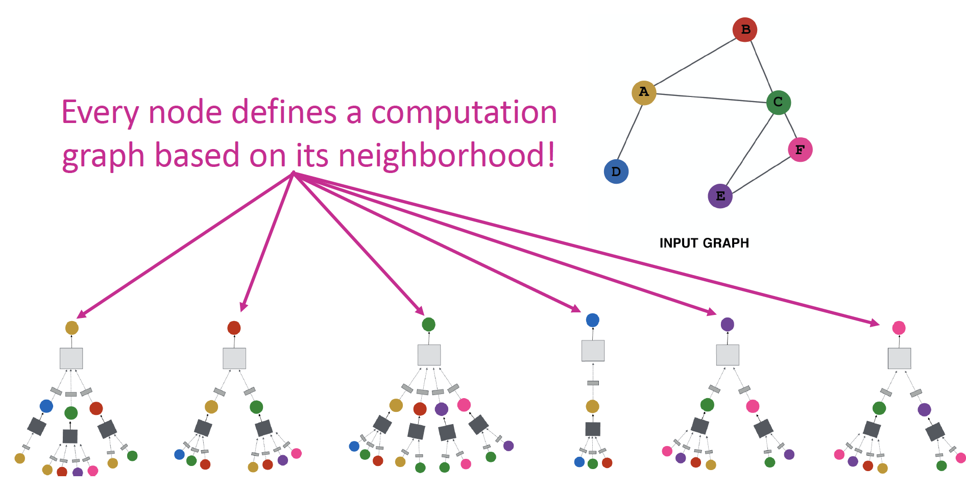
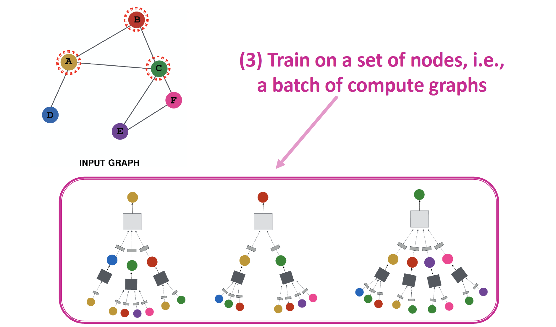
Intuition 2

neighborhood 가 computation graph 를 결정합니다.
모든 node들은 자기 자신만의 Neural Network Architecture 를 갖고 있으며, 각자의 neighborhood에 근거하여 computation graph를 정의합니다.

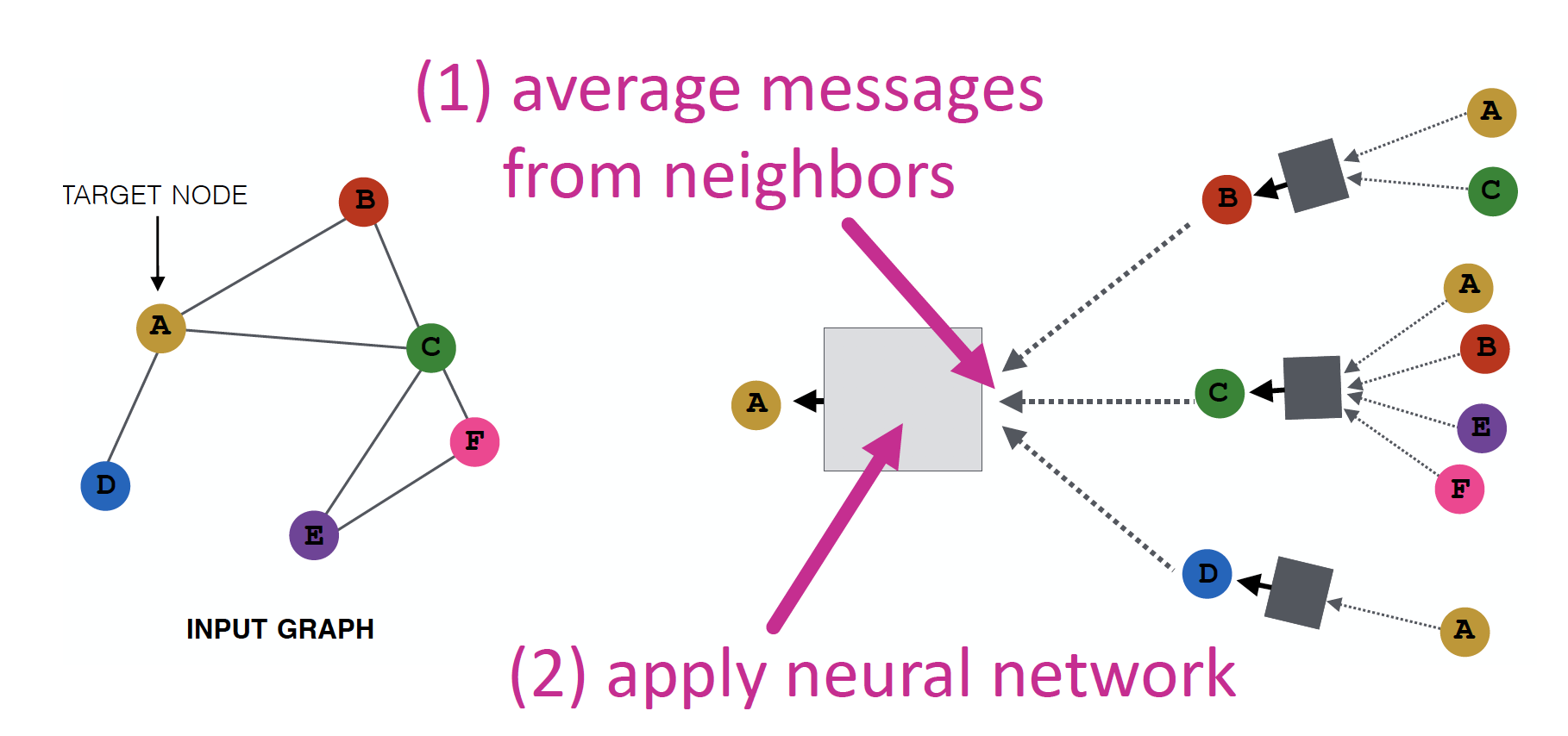
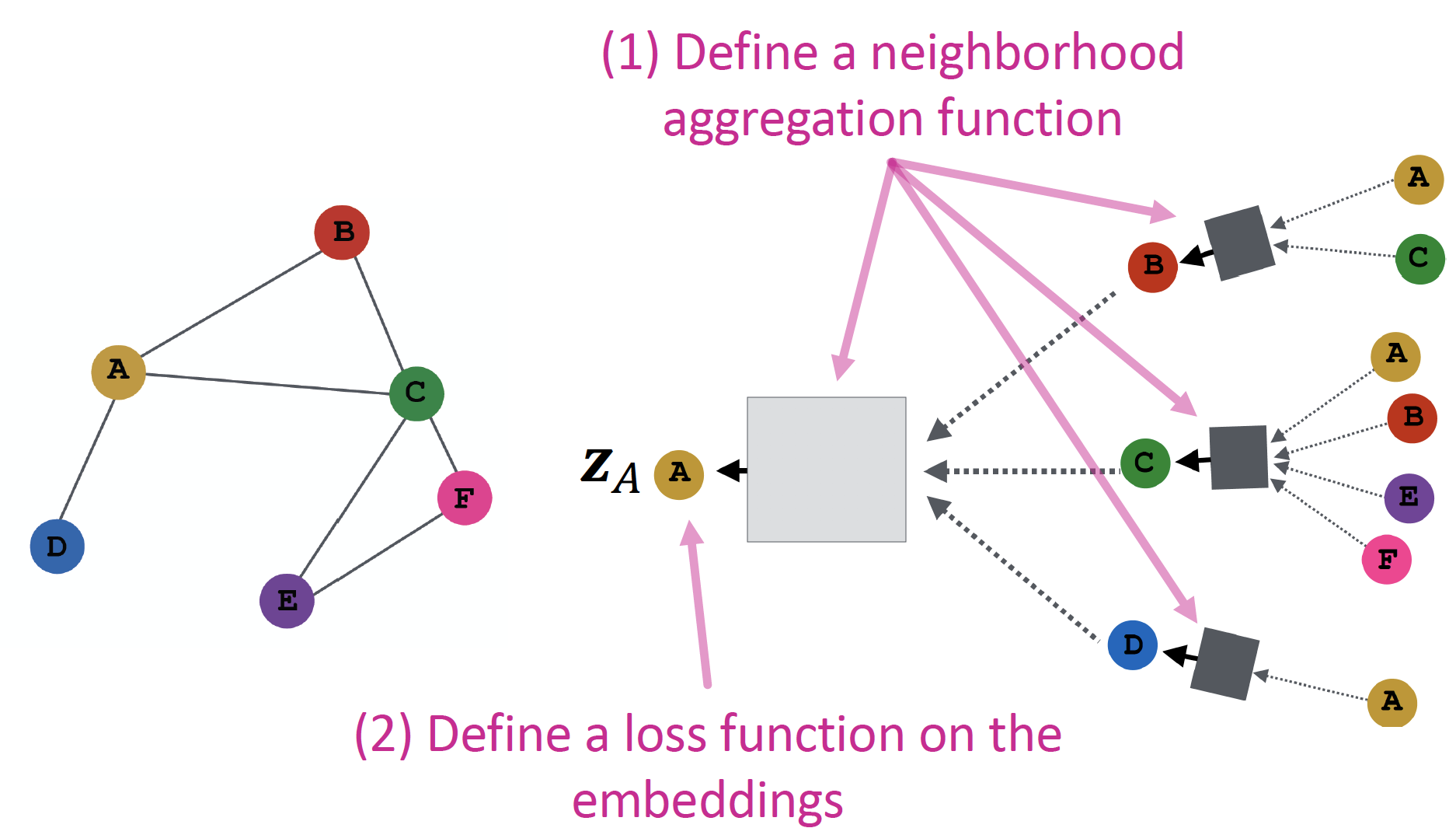
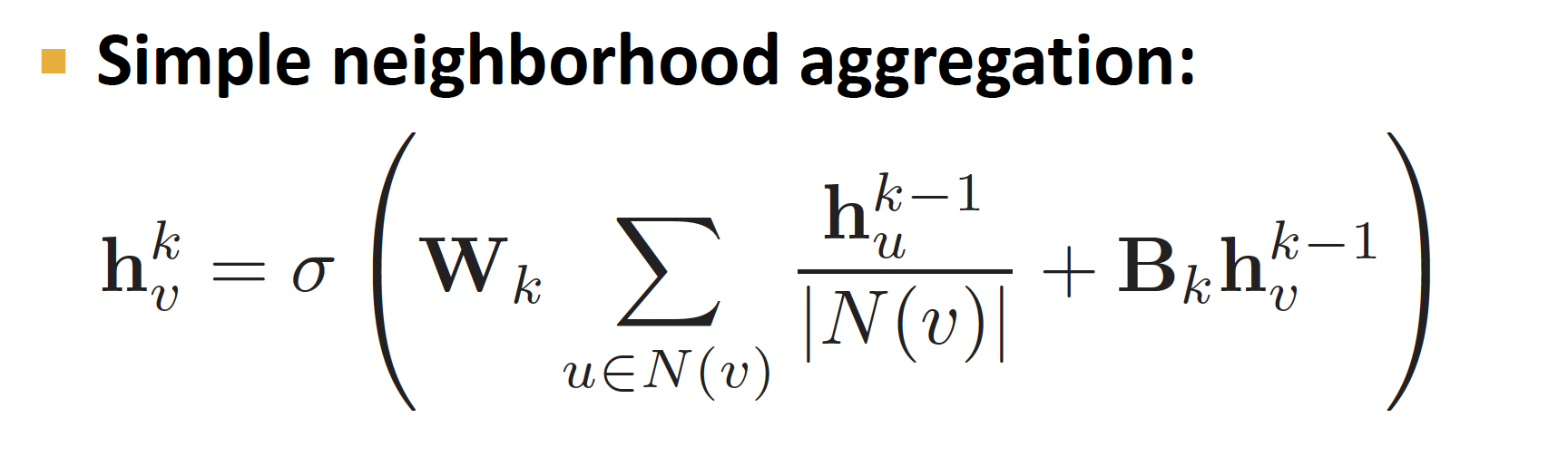
Neighborhood Aggregation

Neighbors 로 부터 정보를 모아 Average 한 뒤, Neural Network 를 적용합니다.

Models

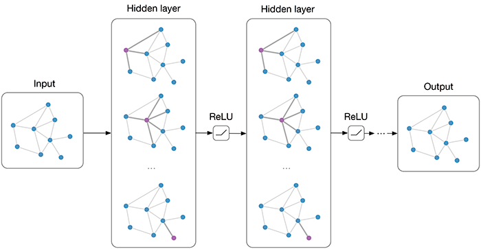
Deep Layer Model

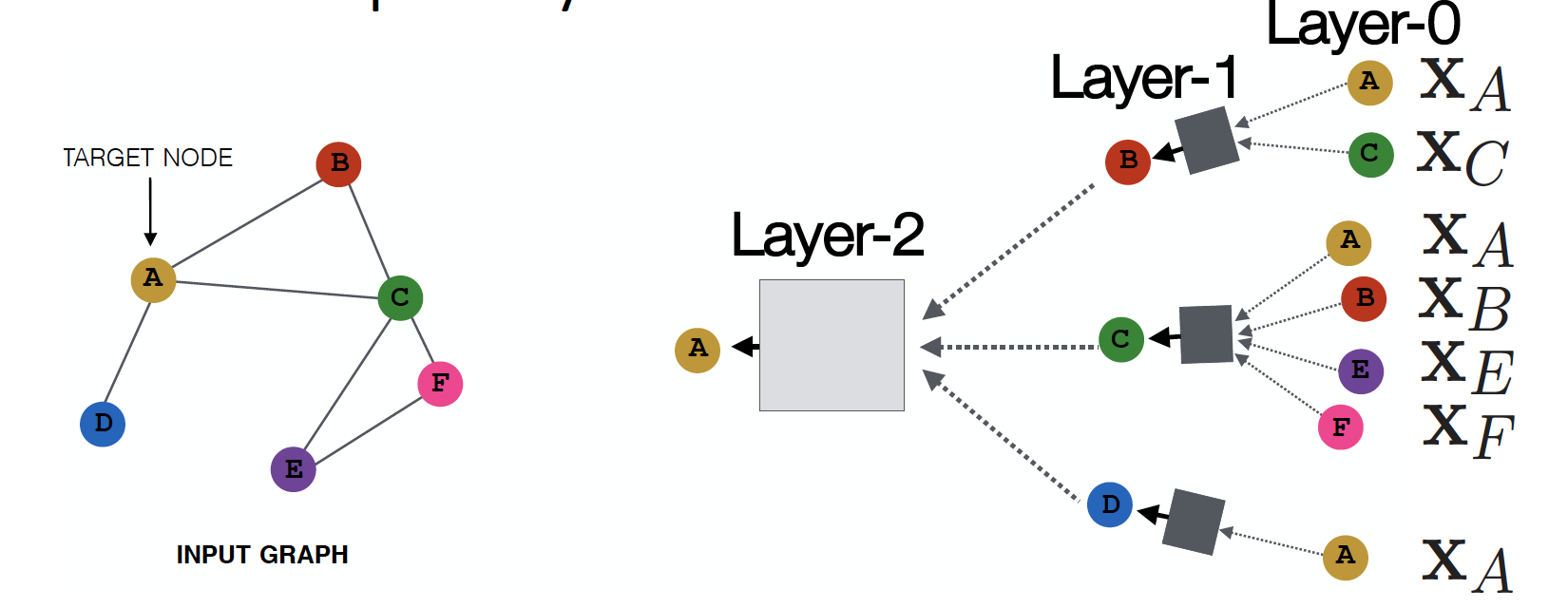
Model의 depth는 자유롭게 설정할 수 있습니다.

• Node는 각 layer에서 embedding 값을 가지게 됩니다.
• Layer-0에서의 node A의 embedding 은 $X_A$ 가 됩니다.
• Layer-K에서의 embedding 은, Layer-0 에서 시작하여 Hidden Layer를 거쳐 K번 전달된 정보에 대한 값을 가지게 됩니다.

Deep Encoder

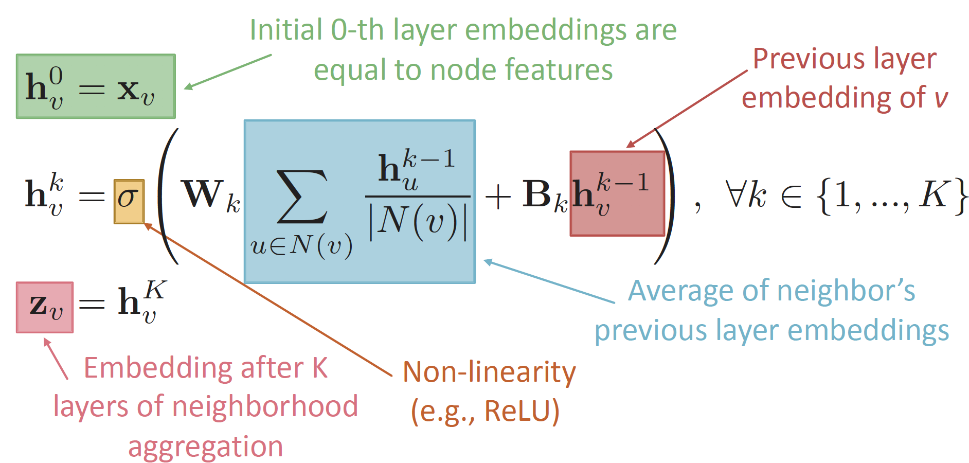
정보가 전달되어 embedding 값을 가지게 되는 과정을 수식적으로 표현하면 위와 같습니다.

• W : Average of neighbor's previous layer embeddings
• B : Message myself from the previous layer

Training the Model

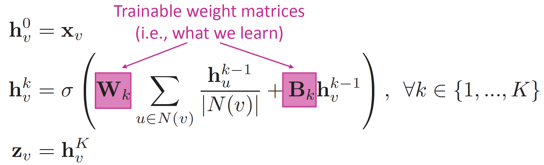
위의 식에서, Train의 대상은 Weight Matrix 인 W 와 B 입니다.
W 와 B 비율을 통해, friend / own property 중 어디에 더욱 주목할 지 결정합니다.

• W ↑ , B ↓ : Neighbor 정보 더욱 많이 고려
• W ↓ , B ↑ : 이전 레이어의 자신의 정보를 더욱 많이 고려

embedding 값은 어떠한 loss function에도 적용 가능하며,
Stochastic Gradient Descent 를 통해 Weight를 update 합니다.

Loss Function은 Task에 따라 달라집니다.

1. Unsupervised Training

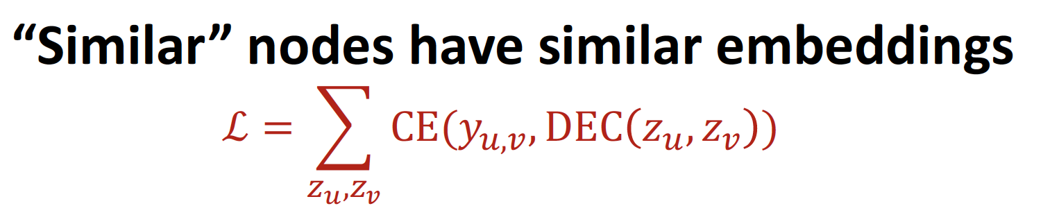
Task : graph structure 를 고려한 node embedding

• node u 와 node v 가 similar 할 때, $y_{u,v} = 1$ 이 됩니다.
• CE : Cross Entropy
• DEC : Decoder (ex. inner product)
• Loss Function : Random Walks, Graph Factorization, Node Proximity in the Graph

2. Supervised Training

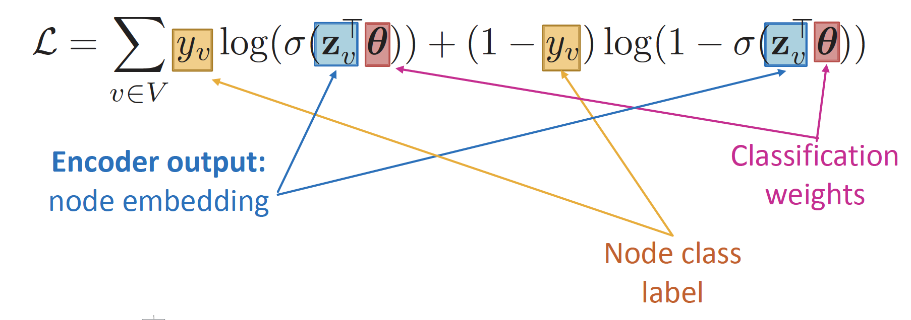
Task : node classification

• Cross Entropy Loss
• $y_v$ : ground-truth label
• Positive node 라면 $\sigma({z_v}^T\theta)$ 값이 커지고, Negative node 라면 $1 - \sigma({z_v}^T\theta)$ 값이 커지게 됩니다.

Overview

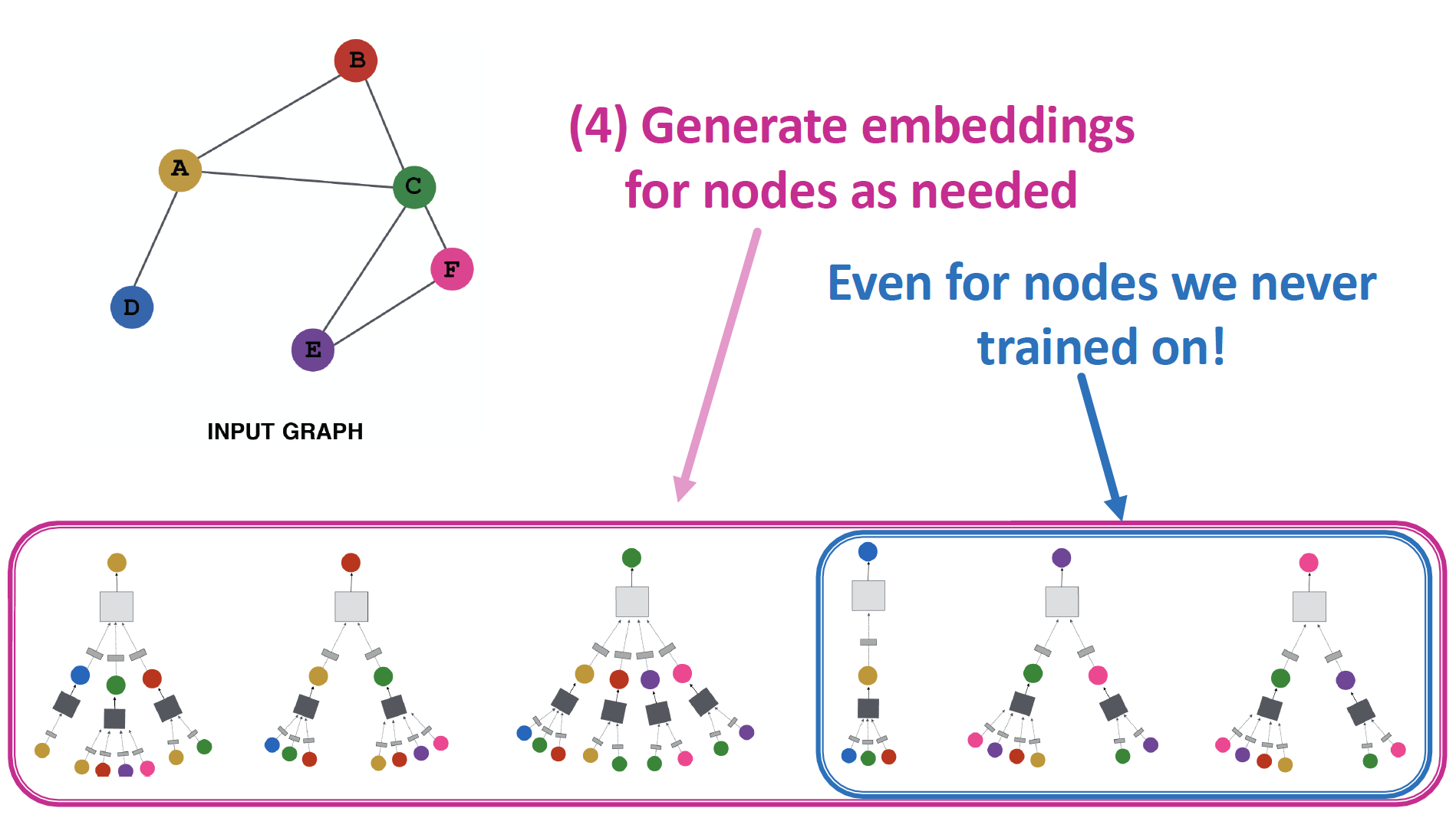
Parameter Sharing

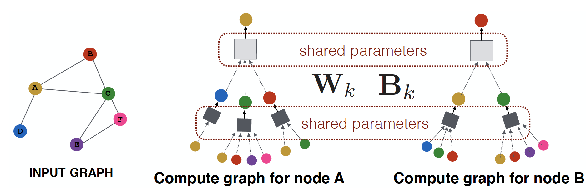
The same aggregation parameters are shared for all nodes
new nodes & new graphs 에 대해서도, generalize 가능합니다.

Summary

Generate node embeddings by aggregating neighborhood information

Graph Neural Network

Layer에서 Neighborhood 와 자기 자신의 message 를 Aggregate 하여 embedding 을 만들고, 이를 전달하여 최종 target node의 embedding 을 만드는 것입니다.

2. Graph Convolutional Network (GCN)

Matrix Formulation

k-1 hidden layer에서 information aggregation을 통해 k hidden layer 로 전달하는 Neighborhood Aggregation 식은 위와 같습니다.

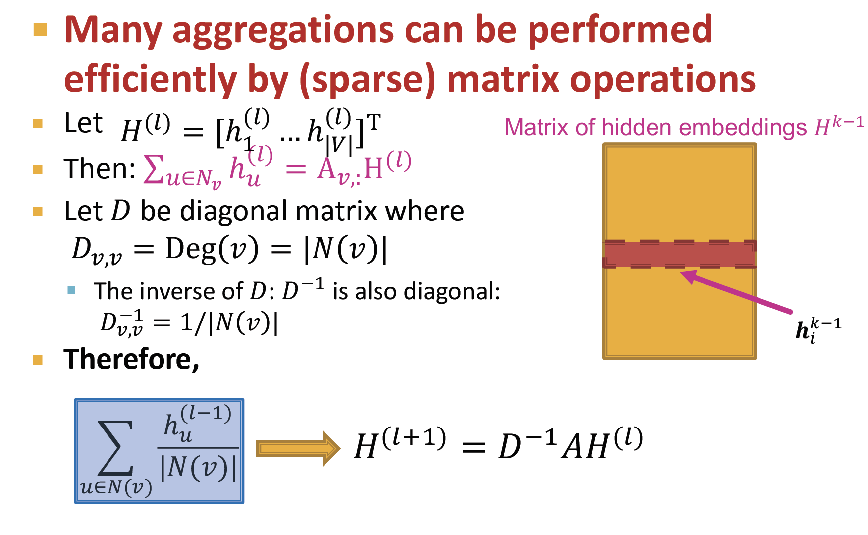
$A$ (인접행렬)은 node 연결 여부에 대한 정보(0/1)를 담고 있는 행렬입니다.
따라서 $AH^{(l)}$ 는 node i 와 relationship이 있는 state 값만 더한 값으로 update 한다는 의미입니다.
여기에 $D^{-1}$을 곱해 row normalized matrix 를 만들어 냅니다.

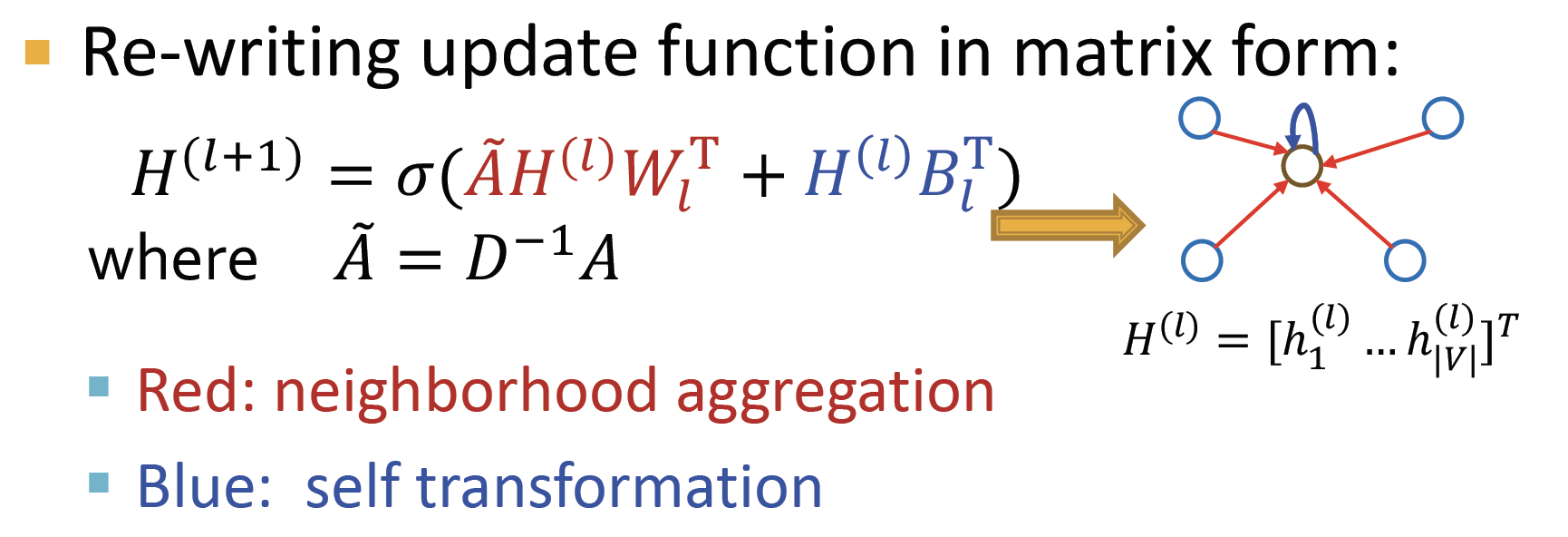
Neighborhood Aggregation 식을 vector form 으로 표현하면 위와 같습니다.

---

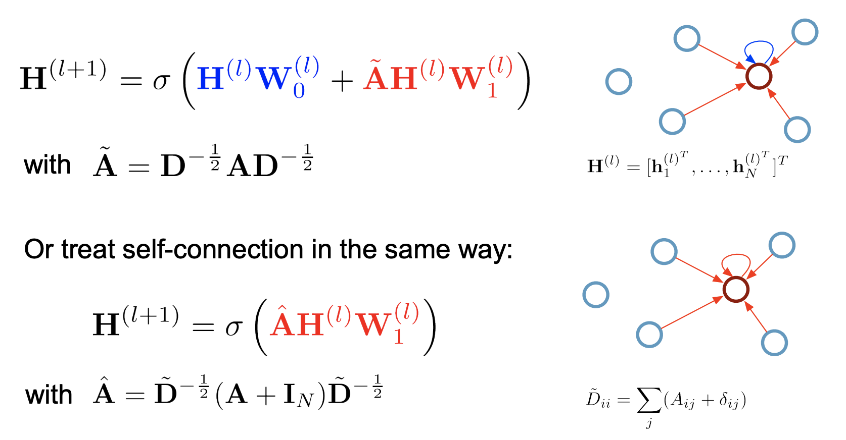
Graph Convolutional Networks

idea

1. neighborhood aggregate 에는 $W_k$ 를 사용하였고, previous self embedding 에는 $B_k$ 를 곱했는데 → GCN 에서는 neighbor 와 self 모두에 대해 동일한 parameter 인 $W_k$ 를 사용합니다.

2. 인접행렬($A$)을 사용하게 되면 자기 자신으로의 연결을 고려하지 않게 되므로 → self-connection을 추가한 $\hat{A} = A + I_N$ 행렬을 사용합니다.

3. 단순히 neighborhood 정보의 평균 ($D^{-1} A$)을 구하지 않고 → neighborhood aggregation 에 symmetric normalization ($D^{-1/2} A D^{1/2}$)을 적용하여 계산합니다.

$f(H^{(l)}, A) = \sigma ({\hat{D}}^{-\frac{1}{2}}\hat{A}{\hat{D}}^{\frac{1}{2}}H^{(l)}W^{(l)})$

1. graph 에서 $\hat{A}$, $\hat{D}$ 를 얻습니다.
2. 각 node에 연결된 edge 개수에 대해 normalization 을 진행합니다.
3. l번째 hidden state 인 $H^{(l)}$ 을 곱합니다.
4. 학습 가능한 parameter $W^{(l)}$ 을 곱합니다.
5. activation function $\sigma$ 를 거쳐 비선형성을 학습합니다.

Output : 인접 노드들의 가중치 $\ast$ feature vector $\ast$ W의 합
즉, GCN은 특정 node의 representation으로, 해당 node에 연결되어 있는 node들을 가중합하는 방법입니다.

---

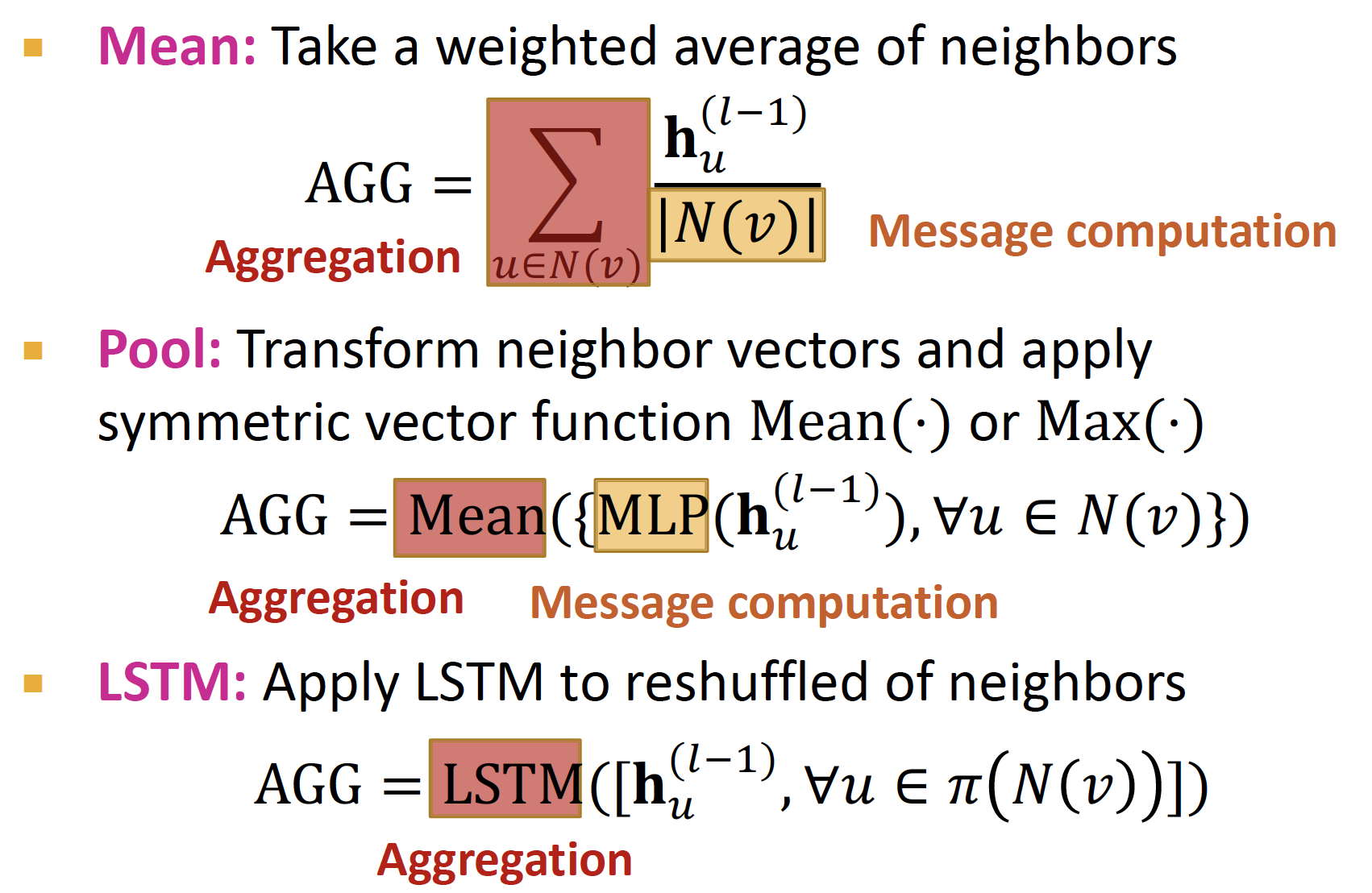
GraphSAGE

idea

1. Concatenate neighbor embedding & self embedding
2. 다양한 Aggregation 방법론을 적용합니다.

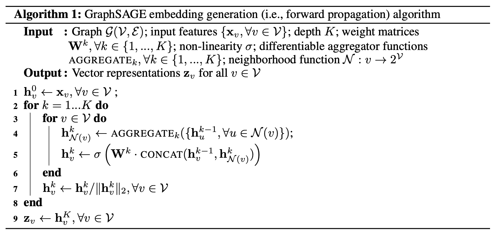
• GCN : neighbor 과 self 의 message 를 더합니다.
  
  GraphSAGE : neighbor 과 self 의 message 를 concat 합니다.
  

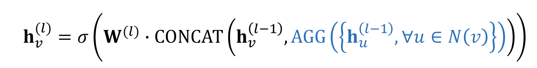
• Aggregation 방법은 여러 가지가 있습니다.
  

3. Graph Attention Network (GAT)

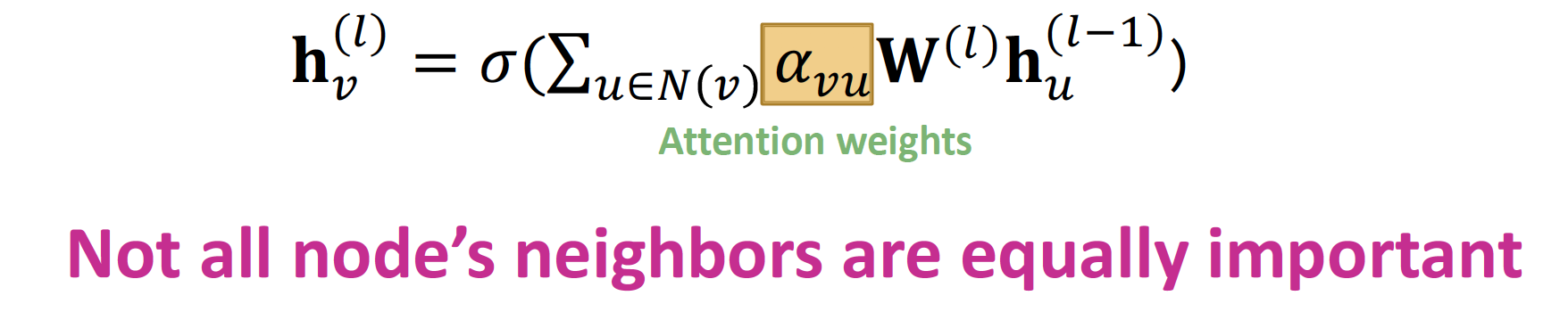
각 neighborhood node들의 중요도를 같다고 보지 않고 ($\neq \frac{1}{|N(v)|}$), attention coefficients $e_{vu}$ 를 적용해 neighborhood node 마다 가중치를 다르게 적용합니다.

Attention Mechanism in NLP

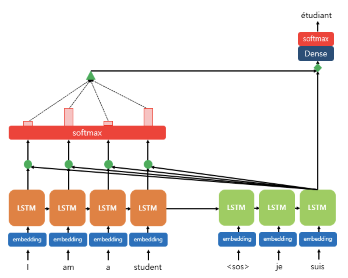
출력 값을 예측할 때, encoder의 모든 입력 단어들의 정보(확률값)를 다시 한번 참고하여 손실했던 정보를 반영합니다.

1. $e^t = [{s_t}^T h_1, {s_t}^T h_2, ... , {s_t}^T h_N]$
   encoder 에서 나온 hidden state 에, 현재 시점 t에서의 decoder hidden state 값을 dot product 연산을 통해 구합니다.
2. $a^t = softmax(e^t)$
   attention distribution 을 구합니다.
3. $a_t = \sum\limits_{i=1}^N a_i^t h_i$
   encoder의 hidden state와 Attention Weights를 곱하고, Weighted Sum 합니다.
4. $v_t$ = concat($a_t$, $s_t$)
   attention value 와 decoder hidden state 값을 concat 한 후, 최종 layer 를 통과하여 output 을 계산합니다.

Attention Mechanism in Graph

PROCESS

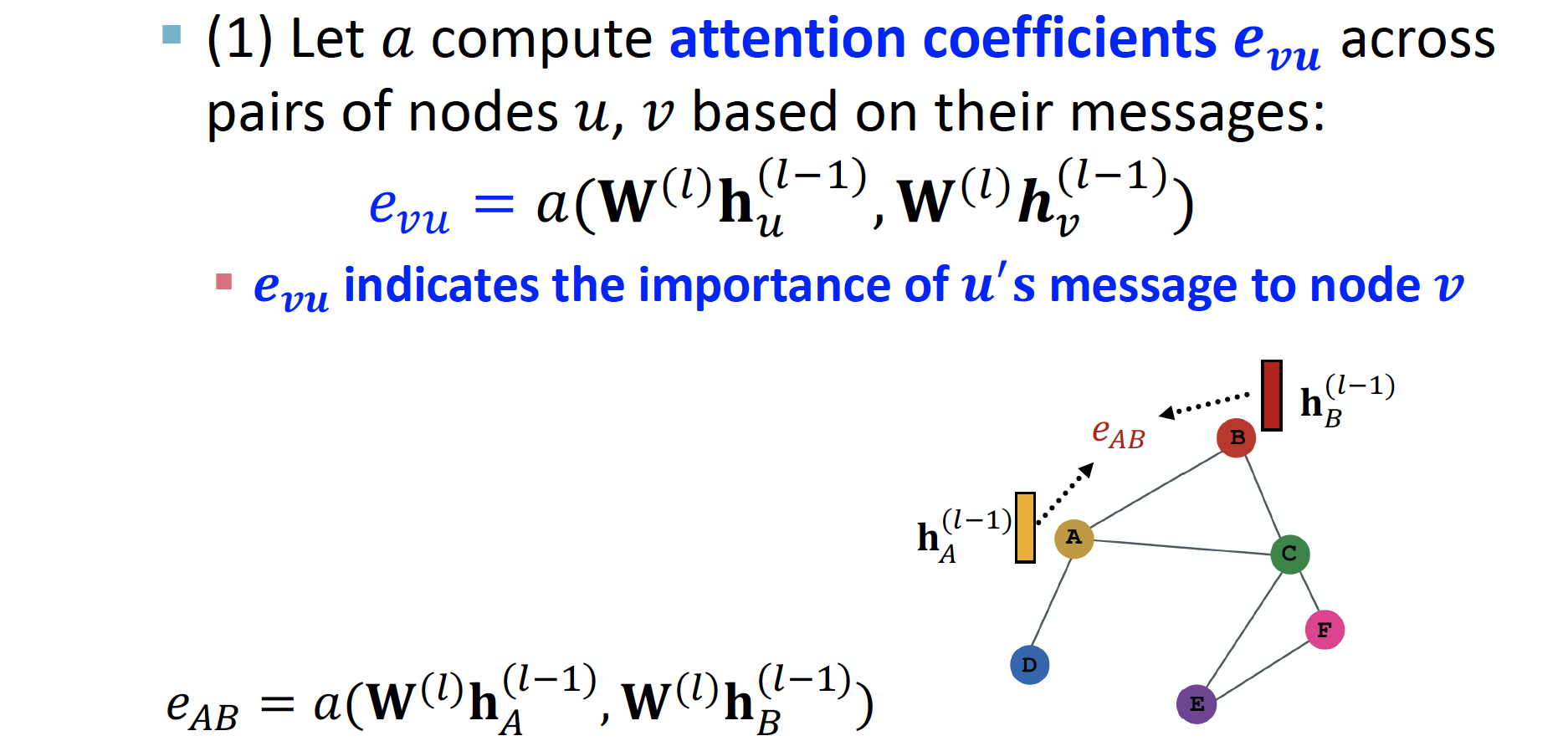
$e_{vu}$ 를 통해서 노드 $u$에서 노드 $v$로 가는 message importance 를 계산합니다.

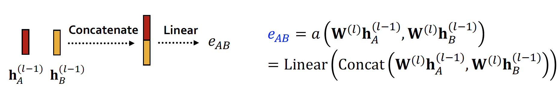
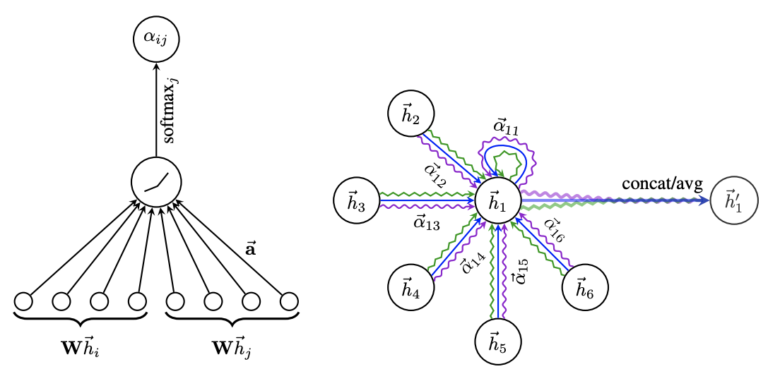
각 node 의 hidden state 값이 concat 되고, linear 를 거쳐 attention coefficient $e_{vu}$ 가 계산됩니다.

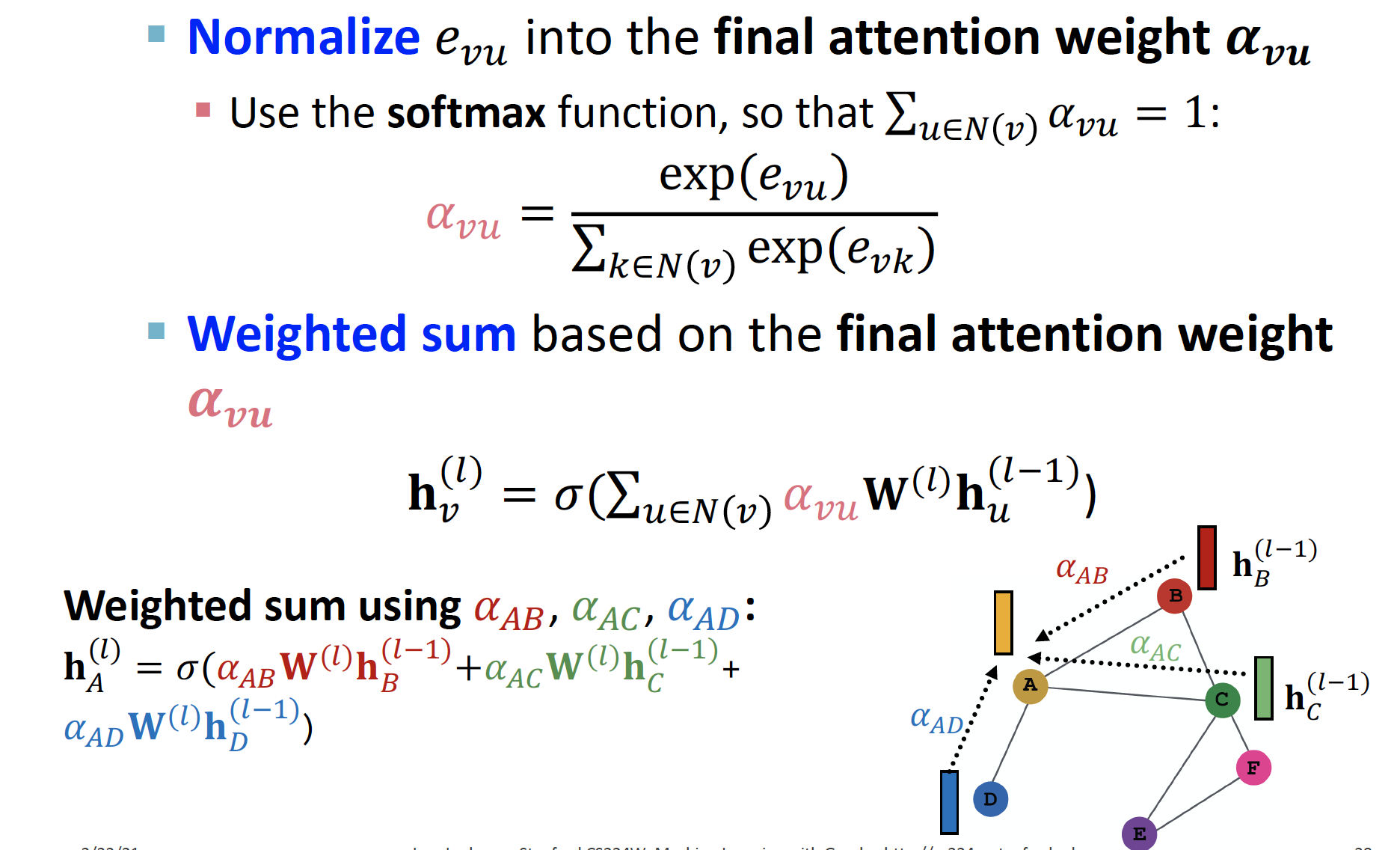
softmax 함수 를 거치고, 이를 통해 나온 값 $\alpha_{vu}$ 을 곱해 가중합 하여 $h_v^{(l)}$ 을 계산합니다.

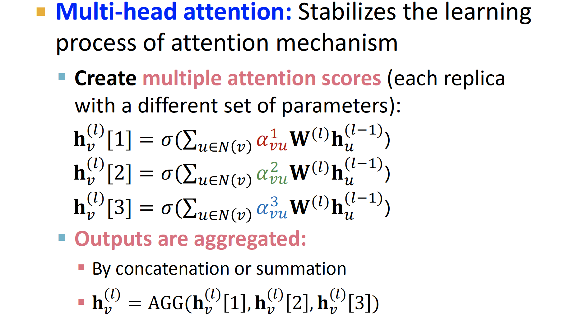
Multi-head attention 을 통해 값을 여러 개 도출하여, 이를 aggregate 해서 최종 output을 계산합니다.
✔︎ Multi-head attention : 서로 다른 attention mechanism을 여러 번 계산하여, input을 여러 관점(head)에서 해석

Allows for (implicitly) specifying different importance values to different neighbors

Experiments

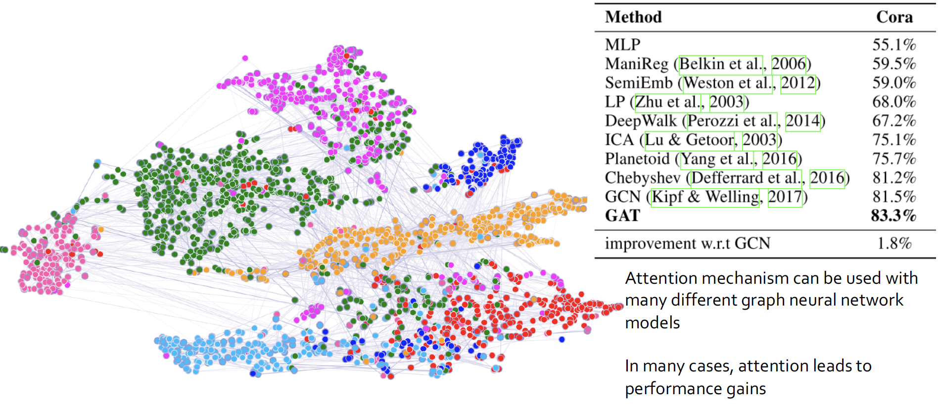
MLP 보다는 Random Walk 가, 이보다는 GCN 과 GAT 가 훨씬 성능이 좋다고 합니다.

4. Application

Pinterest

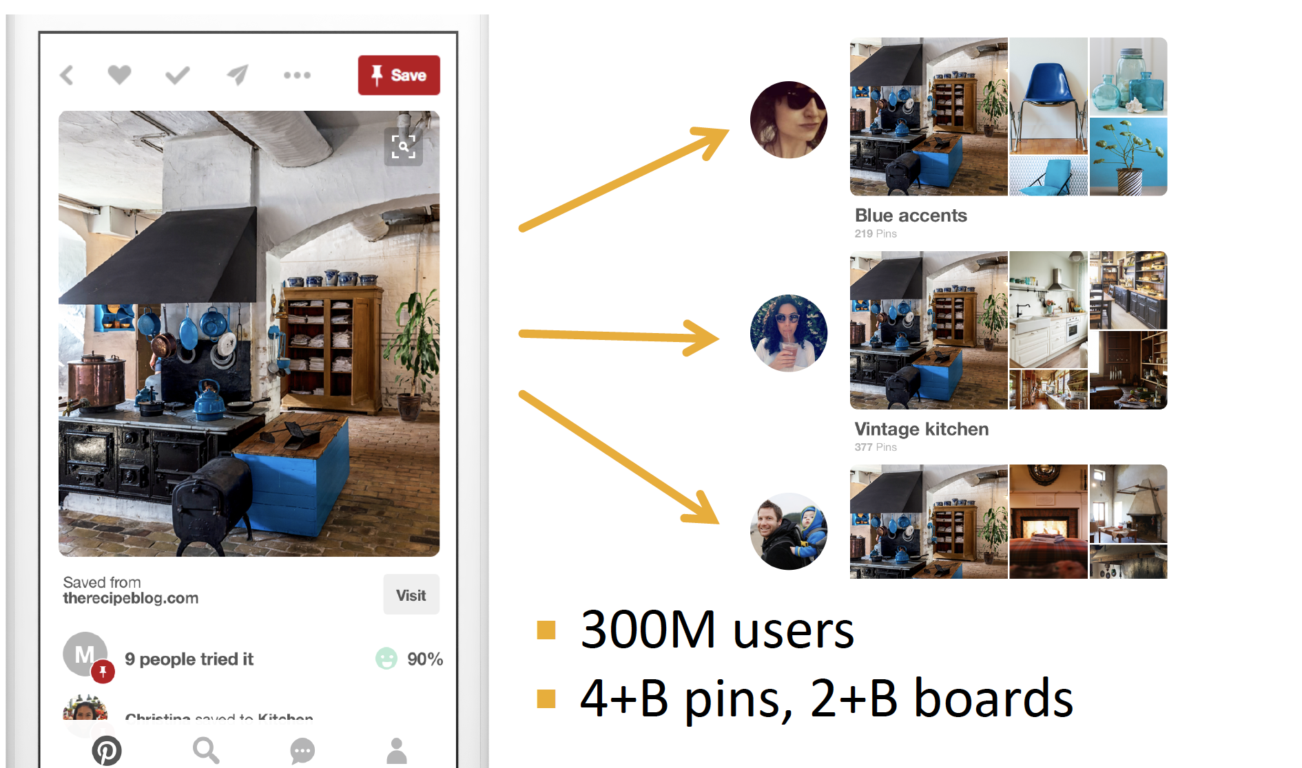
Graph 를 이용해서 더 나은 Recommendation 결과를 도출합니다.

PinSAGE

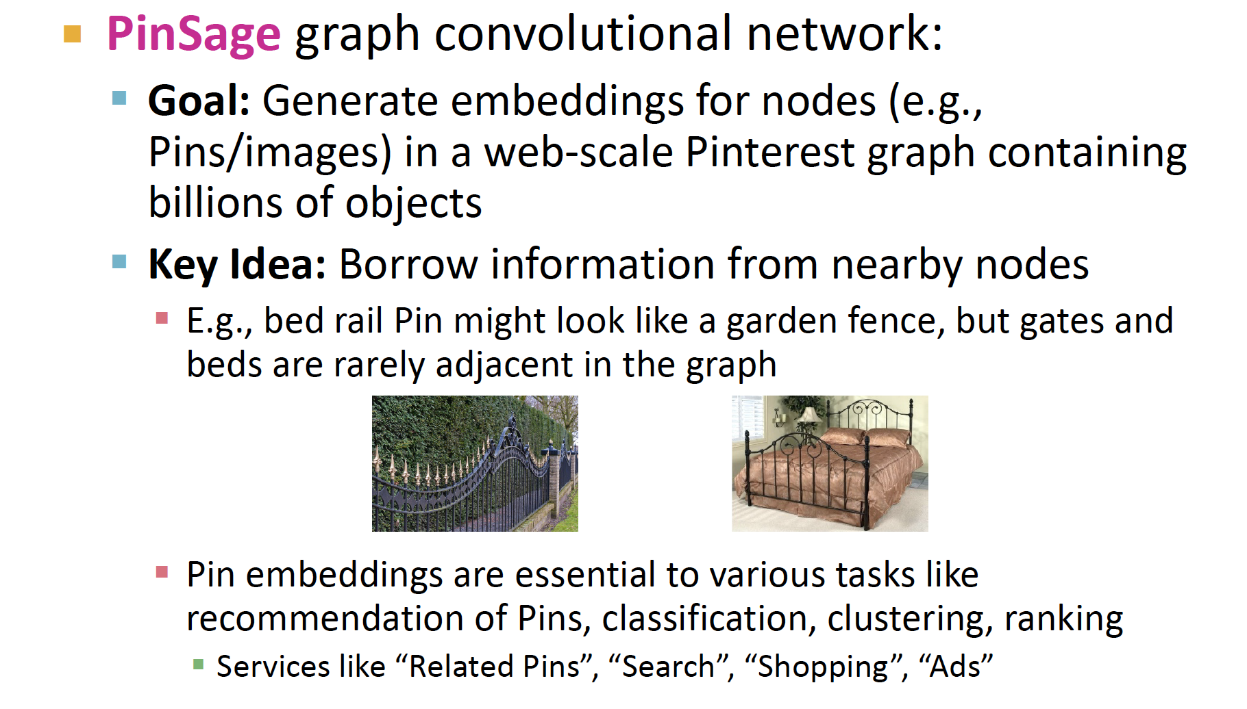
visual 로만 구분하면, fence 와 bed 를 제대로 구분할 수 없게 됩니다.
따라서 Image 와 이를 한 곳에 모아 놓은 Pins 를 node 로 하여, bipartite graph 를 구축해 좀 더 나은 추천 결과를 도출합니다.

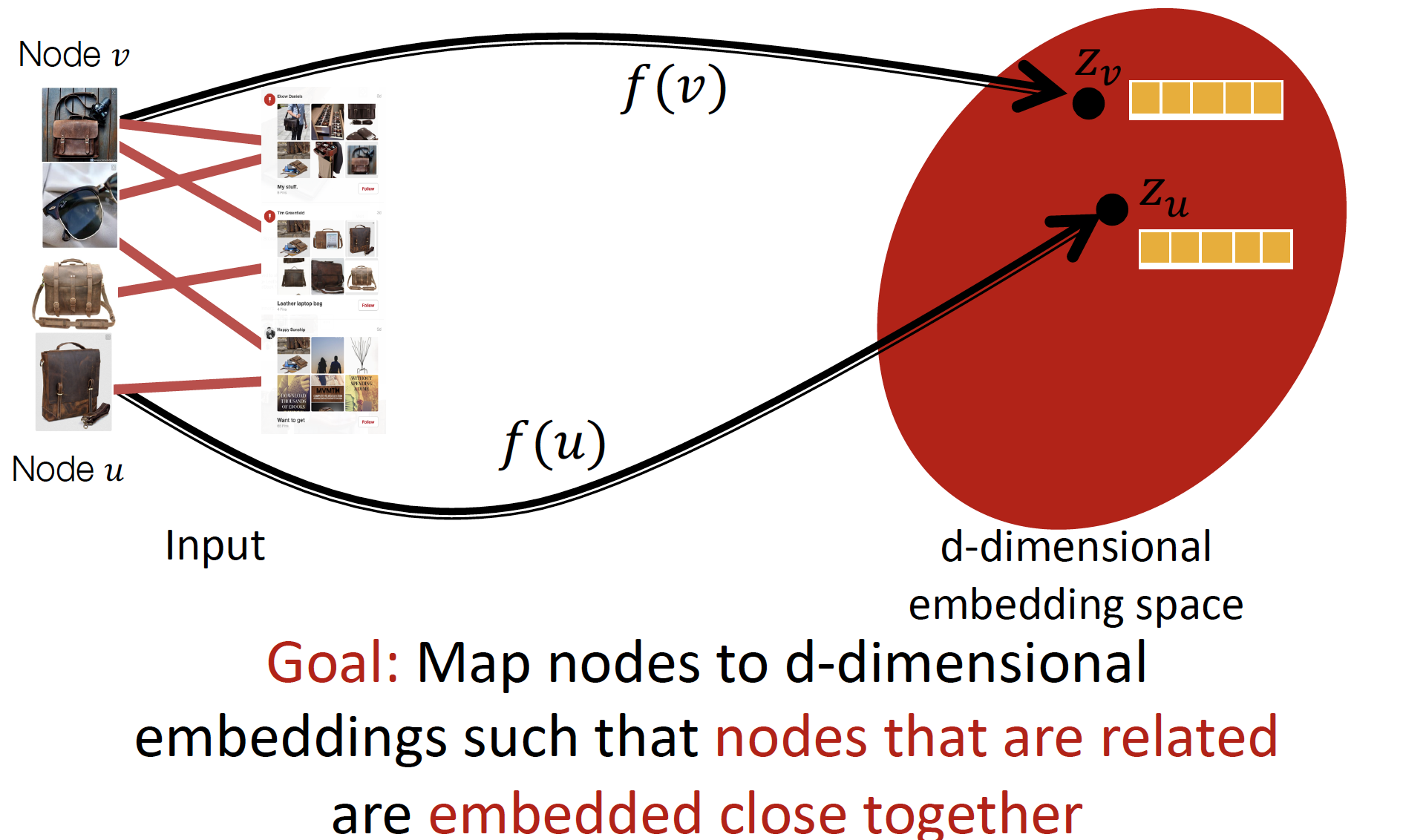
node v image 를 embedding 하여, similar 한 node u 를 찾고, node u의 neighbor 를 추천해 줍니다.

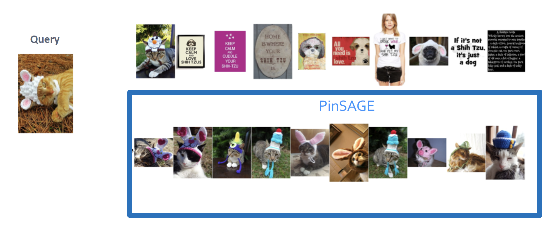
Graph 적용 시 훨씬 좋은 추천 결과를 보인다고 합니다.

Reference

Reviews

1. Tobigs Graph Study : Chapter8. Graph Neural Networks
2. 데이터 괴짜님 Review : CS224W - 08.Graph Neural Networks
3. snap-stanford Review : Graph Neural Networks

---

CS224W Winter 2021

1. Lecture 6. Graph Neural Networks - 1: GNN Model
2. Lecture 7. Graph Neural Networks - 2: Design Space

---

GCN

1. Paper : Semi-Supervised Classification with Graph Convolutional Networks
2. Review : Graph Convolutional Networks
3. PyTorch Code : tkipf/pygcn
4. reference links
5. GraphSAGE : Inductive Representation Learning on Large Graphs

---

GAT

1. Paper : Graph Attention Networks
2. PyTorch Code : Diego999/pyGAT
3. reference links

---

etc.

1. 컨볼루션(Convolution) 이해하기
2. jihoon님 Review : Graph Neural Network
3. Deep Learning on Graphs with Graph Convolutional Networks
4. Interpretation of Symmetric Normalised Graph Adjacency Matrix?
5. lee-ganghee님 Review : GNN, GCN 개념정리
6. wikidocs : 어텐션 메커니즘 (Attention Mechanism)
7. Yeongmin님 GCN Paper Review : Graph Convolutional Networks Review