Abstract

We present high quality image synthesis results using diffusion probabilistic models,
a class of latent variable models inspired by considerations from nonequilibrium
thermodynamics.

이 페이퍼의 핵심은 열역학의 '확산' 개념에서 출발한 diffusion probabilistic model을 통해 high-quality의 이미지 generation이 가능하다는 것을 이론적으로, 경험적으로 보이는 것이다.

Introduction

Deep Generative Models

• GANs, autoregressive models, flows, VAEs.

Diffusion Probabilistic Models

• Parameterized Markov chain trained using variational inference
• Transitions are learned to reverse a diffusion process
  
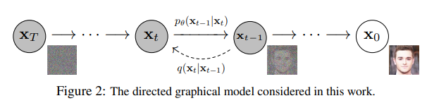
  We hope to learn to reverse of diffusion process.

Diffusion Process?

• Markov chain that gradually adds noise to the data in the opposite direction of sampling.
• Small Gaussian noise for diffusion => Conditional Gaussian for sampling.

Contribution

• First demonstration of generating high quiality samples using diffusion.
• certain parameterization of diffusion models reveals an equivalence
  with denoising score matching over multiple noise levels during training
  and with annealed Langevin dynamics during sampling

BackGround

Diffusion models

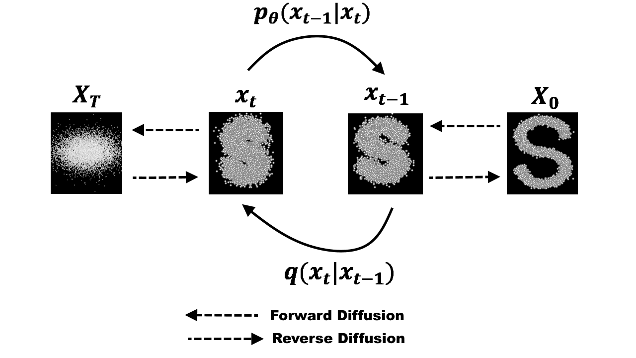
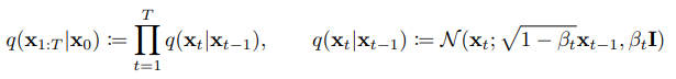
Forward process (diffusion process)

• Approximate posterior $q(\mathbf{x}_{1:T} \mid \mathbf{x}_0)$
• fixed Markov chain that gradually adds Gaussian noise
• Fixed(for this paper) variance schedule $\beta_1, \cdots, \beta_T$
  

Reverse process

• Joint distribution $p_\theta (\mathbf{x}_{0:T})$
• Markov chain with learned Gaussian transitions starting at $p(\mathbf{x}_T) = \mathcal{N} (\mathbf{x}_T ; \mathbf{0}, \mathbf{I})$
  

Optimization goal

• usual variational bound on negative log likelihood
• Related to VAEs (Next topic)
  

Efficient training

• Forward process variances $\beta_T$
• Can be learned by reparameterization, but can be held constant
• if $\beta_T$ is small, the fuctional form of reverse and forward process is same.

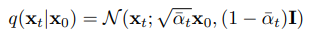
Forward process's property

• $\alpha_t :=1-\beta_t$ , $\bar{\alpha_t} := \prod_{s=1}^t \alpha_s$
  

Rewriting $L$

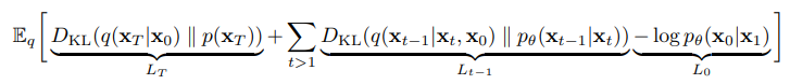
• using KL divergence to directly compare $p_\theta (\mathbf{x}_{t-1} \mid \mathbf{x}_t)$ against forward process posteriors
• tractable when conditioned on $\mathbf{x}_0$
  
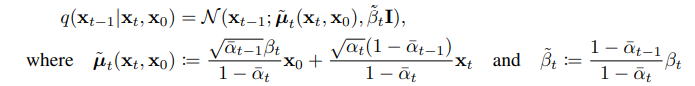
• Can be calculated in a Rao-Blackwellized fashion with closed form expressions
  (since all KL divergences are comparisions between Gaussians)

Diffusion models and denoising autoencoders

Large number of freedom

• $\beta_t$ of forward process
• model architecture
• Gaussian distribution parameterization of reverse process

3.1 Forward process and $L_T$

• $\beta_t$ fixed
• $q$ (approximate posterior) has no learnable parameter
• $L_T$ is constant

3.2 Reverse process and $L_{1:T-1}$

The choices in $p_\theta (\mathbf{x}_{t-1} \mid \mathbf{x}_t) = \mathcal{N} (\mathbf{x}_{t-1} ; \mathbf{\mu}_\theta (\mathbf{x}_t, t), \sum_\theta (\mathbf{x}_t , t))$.

1. $\sum_\theta (\mathbf{x}_t , t) = \sigma_t^2\mathbf{I}$

• to untrained time dependent constants.
• $\sigma_t^2 = \beta_t$ vs $\sigma_t^2 = \tilde{\beta_t} = {1-\bar{\alpha}_{t-1}\over1-\bar{\alpha}_t}\beta_t$
• empirically similar results.
• First one is optimal for $\mathbf{x}_0 \sim \mathcal{N} (\mathbf{0}, \mathbf{I})$
• Second one is optimal for $\mathbf{x}_0$ deterministically set to one point

2. $\mathbf{\mu}_\theta (\mathbf{x}_t, t)$

• specific parameterization motivated by the analysis of $L_t$.

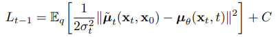
• this means that we should predict $\tilde{\mu}_t$, but using following equations,

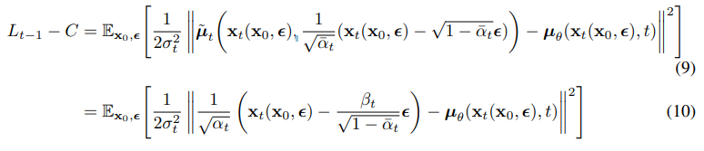
• Equation (10) reveals that $\mathbf{\mu}_\theta$ must predict ${1\over \sqrt{\alpha_t}} \left( \mathbf{x}_t - {\beta_t \over \sqrt{1-\bar{\alpha}_t}}\mathbf{\epsilon} \right)$, meaning that we can train the model to predict $\epsilon$.
  

• The sampling process => resembles Langevin dynamics(랑주뱅 동역학)
  

• 분자 시스템 움직임의 수학적 모델링과 유사한 점을 발견

• Eq(10) simplifies to
  
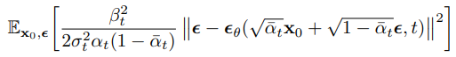
  => resembles denoising score matching over multiple noise scales indexed by t

• https://deepseow.tistory.com/62 참고.

3.3 Data scaling, reverse process decoder, and $L_0$

Assume image data consists of integers in {0, 1, ..., 255} scaled linearly to [-1, 1].
This makes the reverse process operates consistently.

Set the last term of the reverse process to an independant discrete decoder.

• with Gaussian $\mathcal{N} (\mathbf{x}_0 ; \mathbf{\mu}_\theta (\mathbf{x}_1, 1), \sigma_1^2 \mathbf{I})$
  
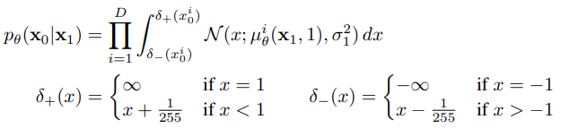
• D is data dim, i is superscript indicating extraction of one coordinate.
• Ensures that the variational bound is a lossless codelength of discrete data.

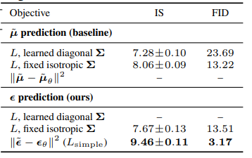
3.4 Simplified training objective

• From above settings, the variational bound is clearly differentiable with respect to $\theta$.
• But, it is beneficial to quality and simpler to implement to train on the following varaint of variational bound.
  
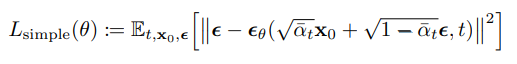
• t=1 case corresponds to $L_0$.
• t>1 case corresponds to unweighted version of $L_t$

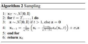
The training can be summarized into:

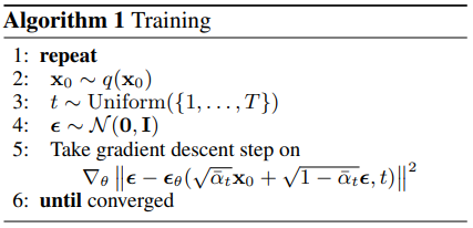
Experiments

• T=1000
• Linearly increasing forward process variances ( $\beta_1 = 10^{-4}$ to $\beta_T=0.02$ )
  - relatively small to data scaled to [-1, 1]
  
• PixelCNN++ as backbone (U-Net based on Wide ResNet)
• Transformer sinusoidal position embedding
• self-attention at 16 $\times$ 16 feature map.
• CIFAR10 model: 35.7M parameters, 10.6 hours to train on 8 V100
• LSUN and CelebA-HQ models: 114M parameters.

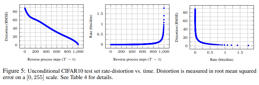
Progressive lossy compression

Progressive generation

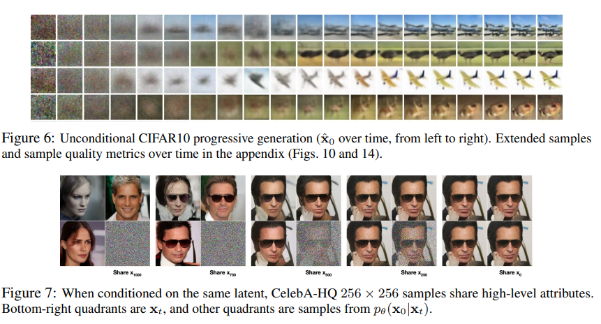
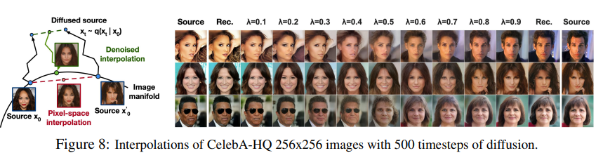
Interpolation