Paint Transformer: Feed Forward Neural Painting with Stroke Prediction

Stroke를 통해서 painting을 재현하는 방식의 논문이다. 특히, 데이터 셋 없이 Self-training pipeline 을 활용하여 만들어 냈다는 점이 인상깊었다.

Abstract

Neural Painting

Procedure of producing a series of strokes for a given image + non-photo realistic recreation using NN.

RL?

Can generate a stroke sequence step by step
But, training stable RL agents is not easy.

Iterative stroke optimization methods

Stroke optimization methods search for as set of stroke parameters "iteratively" in a large search space, making it less efficient.

Paint Transformer

A novel Transformer-based framework that predicts the parameters of a stroke set with as FFN.
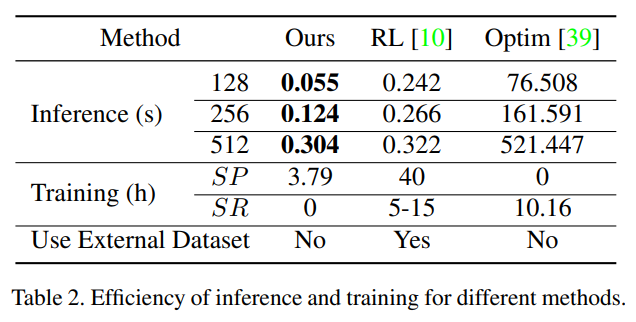
It can generate a set of strokes in parallel and obtaion the final painting of size 512 X 512 in near real time.

Self-training pipeline

No dataset is available for training of the Paint Transformer.
The researchers created self-training pipeline that can be trained w/o any off-the-shelf dataset.
With cheaper traning and inference costs, the methode achieves better painting performance.

Introduction

The goal of this paper seems to be creating a human-creation-like painting, since humans draw painting by stroke-by-stroke procedure. Especially for painting with oil paint or watercolor, the generated paintings can look more like real human.

Previous works

RNN

1. Sequential process of generating strokes 1-by-1
2. Referred to Sketch-RNN

Step-wise greedy search

1. Sequential process of generating strokes 1-by-1

RL

1. Sequential process of generating strokes 1-by-1
2. Pros: Inference is fast
3. Cons: Long training time, Unstable agents

Stroke parameter searching

1. iterative optimization
2. Pros: results are attractive
3. Cons: not enough efficiency and effectiveness.

Overview

Stroke set prediction instead of stroke sequence generation.
Given (initial canvas & target natural image) => predicts set of strokes and render them on the initial canvas to minimize the difference between the rendered image and target one.
This is repeated at K coarse-to-fine(coarse parameter set -> finer parameter set close to the best one in coarse set) scales.
The initial canvas is the output of the previous scale.

The paper suddenly comes with a new concept here.

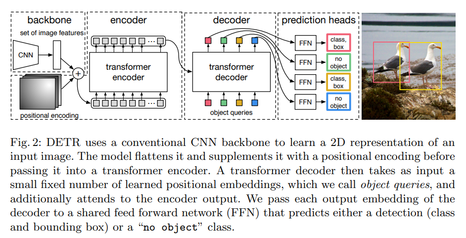
Set prediction problem? => Object detection!

DETR (DEtection TRansformer)

On paper "End-to-end object detection with transformers (2020)" by Facebook AI.

Lack of Data

Unlike object detection, annotated data is unavailable.
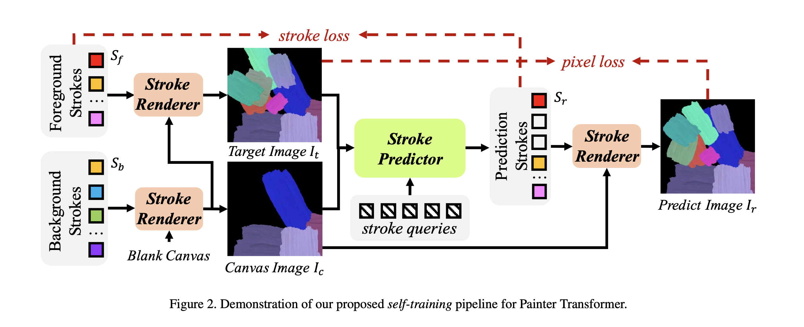
The authors propose a novel self-training pipeline of following steps which utilizes synthesized stroke image.
1. Synthesize a background canvas image with some randomly sampled strokes.
2. Randomly sample a foreground stroke set, and render them on canvas image to derive a target image.
This way, the predictor predicts the foreground stroke set, and the training objective becoms minimizing the difference between synthesized canvas image and the target image.
The optimization is conducted on both stroke and pixel level.

Related Works

Stroke Based Painting

RNN and RL in sequential manner

Object Detection

Recent paper of DETR, performs set prediction w/o post-processing (as non-max suppression)

Methods

Overall Framework

Paint Transformer consists of two modules: Stroke Predictor and Stroke Renderer.

Their relation can be expressed like:

Stroke Predictor

Input: $I_t$(target image) & $I_c$(intermediate canvas image)
Generate: Set of parameters to determine current stroke set $S_r$
Trainablity?: Contains trainable parameters

Stroke Renderer

Input: $S_r$ & $I_c$
Output: Resulting image $I_r$ ($S_r$ drawn onto $I_r$).
Trainablity: Parameter free, differentiable module.

Self-training pipeline (stroke-image-stroke-image)

It uses randomly synthesized strokes, so that we can generate infinite data for training and do not rely on any off-the-shelf dataset.
The training iterations is as following.
1. Ramdomly Sample $S_f$(foreground stroke set) and $S_b$(background stroke set)
2. Generate $I_c$ with $StrokeRenderer(S_b)$
3. Produce $I_t$(target image) by rendering $S_f$ onto $I_c$.
4. $S_r = StrokePredictor(I_c, I_t)$
5. $I_r = StrokeRenderer(S_r, I_c)$

Training objective

$\mathcal{L}_{stroke}$ is stroke loss, and $\mathcal{L}_{pixel}$ is pixel loss.

Stroke definition and Renderer

A stroke $s$ can be denoted as {$x,y,h,w,\theta,r,g,b$} and we consider only straight stroke.

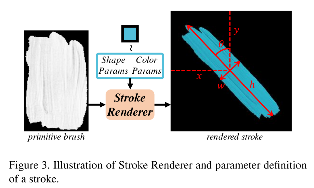
Stroke Renderer

• Geometric transformation based (no NN)
• differentiable (enabling end-to-end learning of Stroke Predictor)
• whole process can be achieved by linear transformation
  $I_{out} = StrokeRenderer(I_{in}, S) \text{ (}S = \{s_i\}^n_{i=1})$
  With a primitive brush $I_b$ and a stroke $s_i$, we can draw the stroke like Fig.3, obtaining $\bar{I^i_b}$.
  $\alpha^i$ is defined as
• binary mask of $s_i$
• generated single-channel alpha map
• same shape with $\bar{I^i_b}$
  Denoting $I_{mid}^0 = I_{in}$,
  The stroke rendering process is like this:
  $I_{mid}^i = \alpha^i \cdot \bar{I^i_b} + (1- \alpha^i) \cdot I^{i-1}_{mid}$
  Output of the stroke renderer is $I_{out} = I_{mid}^n$.

Stroke Predictor

The goal of stroke predictor is to predict a set of strokes that can cover the difference between $I_c$ and $I_t$.
The authors hoped for few strokes prediction while covering most of the differences.

$S_r = StrokePredictor(I_c, I_t)$

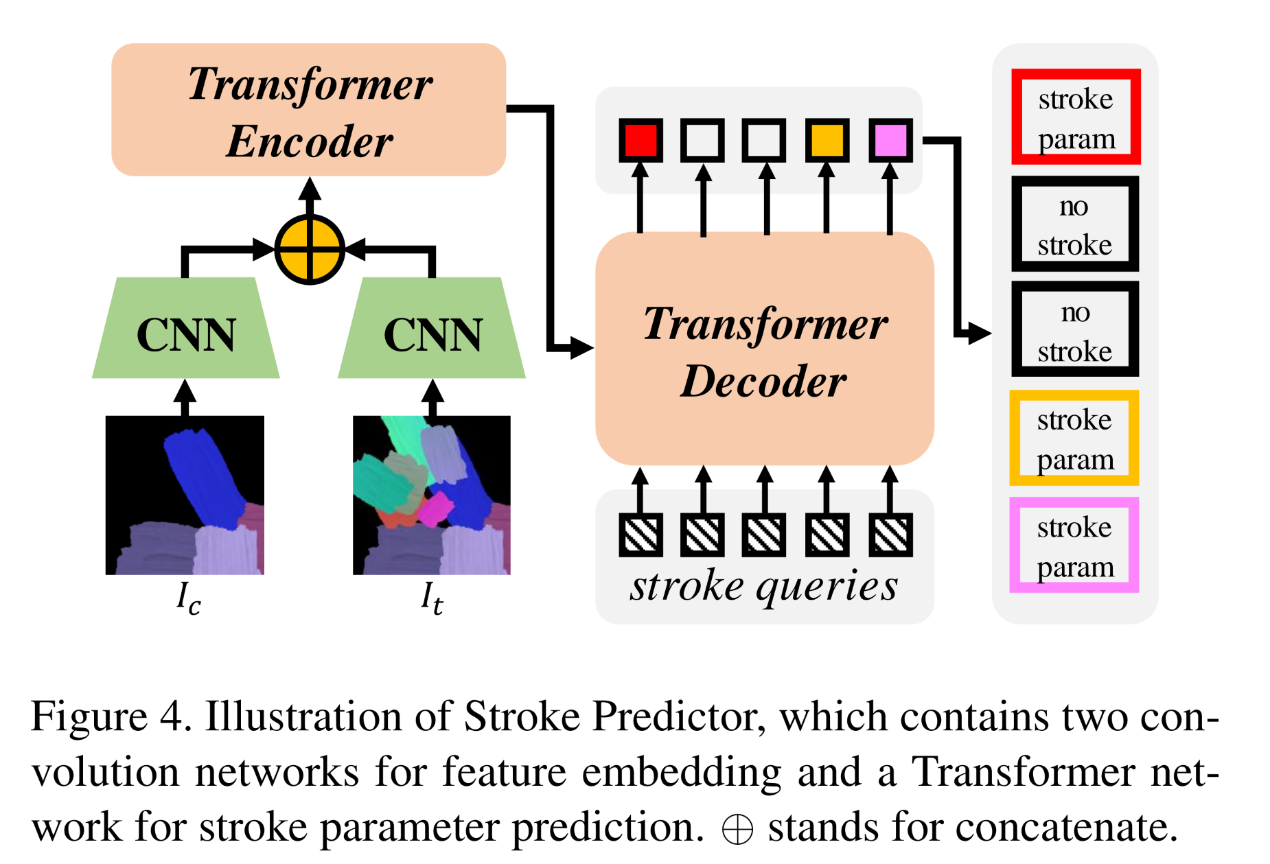
1. Input: $I_c, I_t \in \mathbb{R}^{3\times P \times P}$
2. 2 CNNs: Extract feature maps as $F_c, F_t \in \mathbb{R}^{3\times P/4 \times P/4}$
3. Encoder: $F_c, F_t$ and a learnable positional encodings are concatenated and flattened as the input of Transformer Encoder.
4. Decoder: Use N learnable stroke query vectors as input.
5. 2 branches of Fully-connected layers to predict
   1. $\bar {S_r} = \{s_i\}^N_{i=1}$ (initial stroke params)
   2. $C_r = \{c_i\}^N_{i=1}$ (stroke confidence)
      • convert to a decision $d_i = Sign(c_i)$.
      • $Sign(x)=1\text{ }if \text{ }x>=0, else \text{ }0$
      • $d_i$ is used to determine whether a stroke should be plotted in canvas.
      • Special form in backward phase due to back propagation.

Loss Function

Loss consists of pixel loss and stroke loss.

Pixel Loss

Stroke Loss

$L_1$ metric: dismisses different scales for big and small strokes
$\mathcal{D}_W$ metric: Wasserstein distance (related to rotation)
$\mathcal{D}_{bce}$ metric: BCE of decisions.
$X, Y$: optimal permutations for predicted strokes.

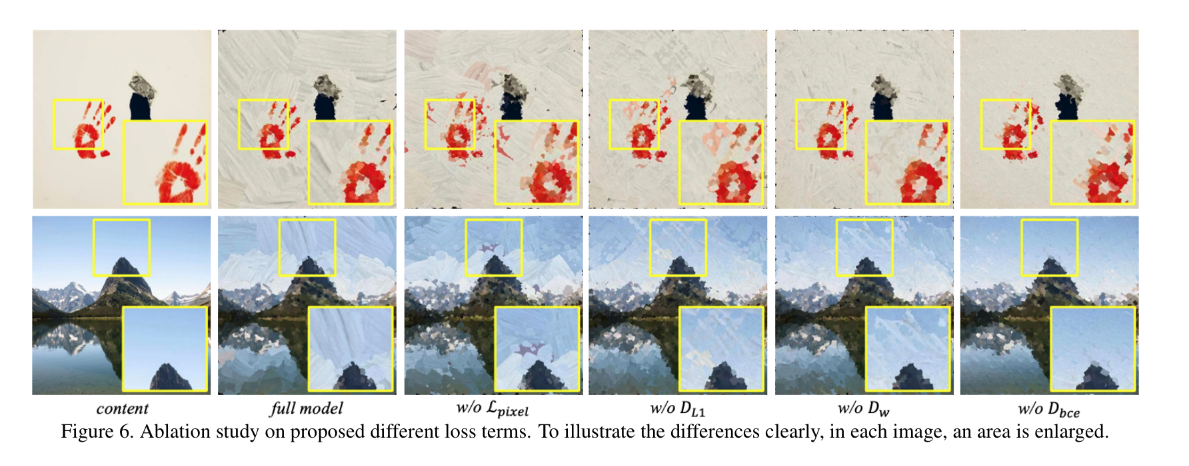
Inference

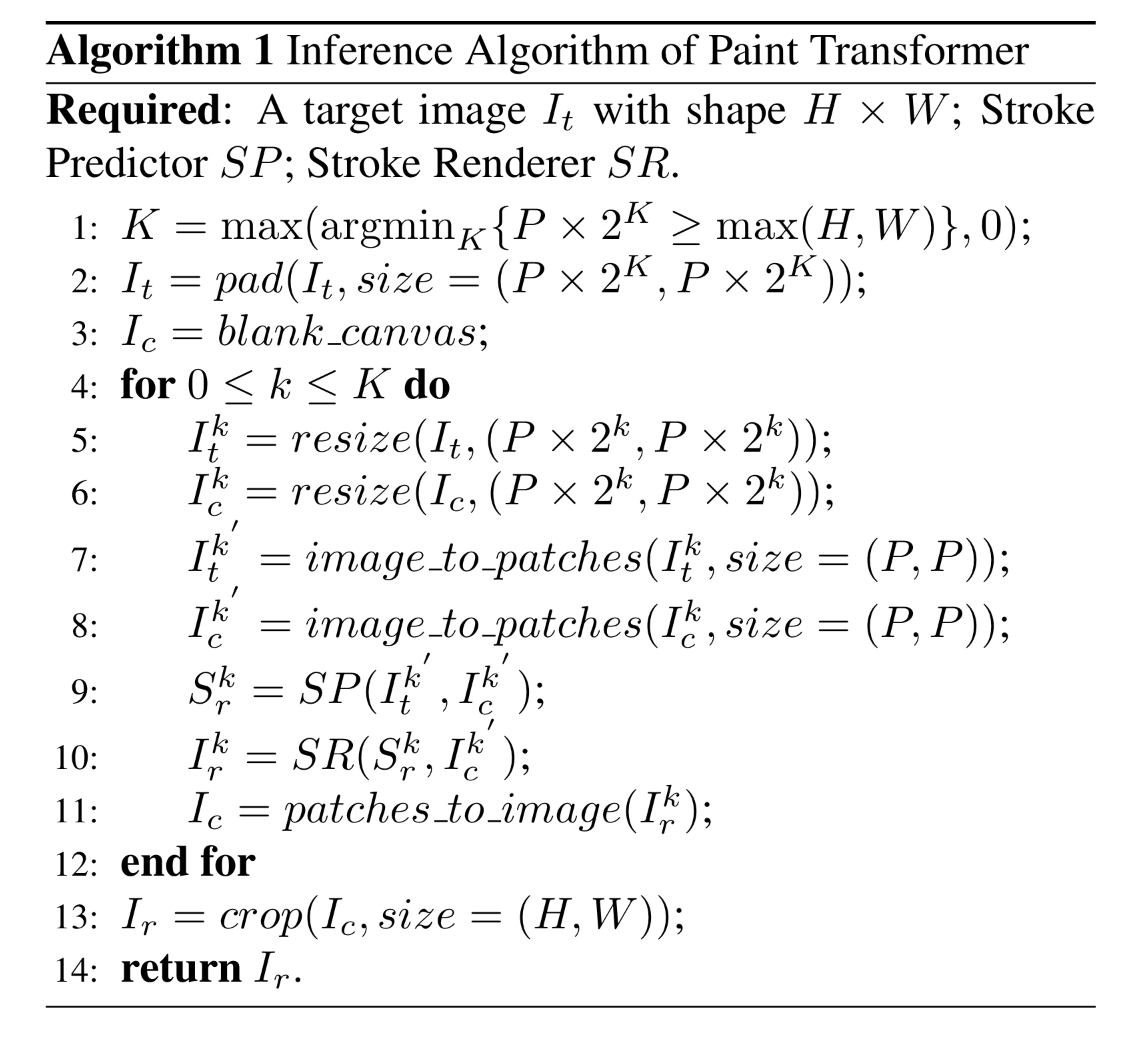
Experiments

Implementation details

• Size $P=32$
• CNNs: 3X[Conv-BatchNorm-ReLU]
• Transformer: $D=256$, 3 layers for encoder and decoder each.
• Training time: 4 hours on 2080Ti.

Comparison