Feature Scaling in Scikit Learn

Data Preprocessing is not just about encoding the data and converting the data type within the dataset. It also requires arduous steps to adjust the widening range of different independent variables hence enabling to exercise similar extent of impact to the model.

Imagine two different features height and weight. It will simply be "nonsensical" to extract meaningful outcome by comparing features with diifferent units (ex - cm vs. kg , ft vs. lb). A process of normalizing the range of variables is called feature scaling.

Feature Scaling

method used to normalize the range of independent variables or features of data (ex- Standardization, Normalization)

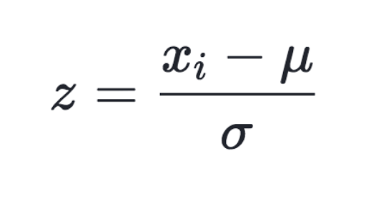
Standardization

a process of converting data feature to have normal distribution of mean of 0 and variance of 1

Normalization

a proecess of converting feature data with different size in a range of [0,1] (i.e - largest value equals 1, while smallest equals 0)

StandardScaler (Standardization)

StandardScaler is a class to provide standardized feature scaling for independent variables (i.e- mean of 0, variance of 1).

First, let us see the average and variances of feature data from the iris sample.

from sklearn.datasets import load_iris
import pandas as pd

iris = load_iris()
iris_data = iris.data
iris_df = pd.DataFrame(data=iris_data, columns=iris.feature_names)

print('Average of Feature')
print(iris_df.mean())
print('\n Feature Variance')
print(iris_df.var())

Output

Average of Feature
sepal length (cm)    5.843333
sepal width (cm)     3.057333
petal length (cm)    3.758000
petal width (cm)     1.199333
dtype: float64

 Feature Variance
sepal length (cm)    0.685694
sepal width (cm)     0.189979
petal length (cm)    3.116278
petal width (cm)     0.581006
dtype: float64

Now, we will use StandardScaler() class to standardize every features.

from sklearn.preprocessing import StandardScaler

# create StandardScaler() object
scaler = StandardScaler()

# fit() & transform()
scaler.fit(iris_df)
iris_scaled = scaler.transform(iris_df)

# transform() returns ndarray -> convert to dataframe
iris_df_scaled = pd.DataFrame(data=iris_scaled, columns=iris.feature_names)
print('Feature Average')
print(iris_df_scaled.mean())
print(' \nFeature Variance')
print(iris_df.var())

Output

Feature Average
sepal length (cm)   -1.690315e-15
sepal width (cm)    -1.842970e-15
petal length (cm)   -1.698641e-15
petal width (cm)    -1.409243e-15
dtype: float64
 
Feature Variance
sepal length (cm)    0.685694
sepal width (cm)     0.189979
petal length (cm)    3.116278
petal width (cm)     0.581006
dtype: float64

The averages and variances of the data have been converted to values close to 0 and 1 respectively.

MinMaxScaler (Normalization)

MinMaxScaler converts feature data to a range of [0,1].

# Min Max Scaler 
from sklearn.preprocessing import MinMaxScaler

# create MinMaxScaler() object
scaler = MinMaxScaler()

# fit() & transform()
scaler.fit(iris_df)
iris_scaled = scaler.transform(iris_df)

# transform() returns ndarray -> convert to dataframe
iris_df_scaled = pd.DataFrame(data=iris_scaled, columns=iris.feature_names)
print('Feature Average')
print(iris_df_scaled.mean())
print('\nFeature Variance')
print(iris_df_scaled.var())

print('\nMin Value')
print(iris_df_scaled.min())
print('\nMax Value')
print(iris_df_scaled.max())

Output

Feature Average
sepal length (cm)    0.428704
sepal width (cm)     0.440556
petal length (cm)    0.467458
petal width (cm)     0.458056
dtype: float64

Feature Variance
sepal length (cm)    0.052908
sepal width (cm)     0.032983
petal length (cm)    0.089522
petal width (cm)     0.100869
dtype: float64

Min Value
sepal length (cm)    0.0
sepal width (cm)     0.0
petal length (cm)    0.0
petal width (cm)     0.0
dtype: float64

Max Value
sepal length (cm)    1.0
sepal width (cm)     1.0
petal length (cm)    1.0
petal width (cm)     1.0
dtype: float64

The data have been correctly adjusted to have range of [0,1].

Problem of Scaling Train and Test Dataset

The purpose of feature scaling is to unify the range of feature datasets and avoid any misinterpretation of data of model. When splitting train and test dataset, it is important to maintain identical scaling range for two datasets.

First, we will create two different arrays train_array and test_array to create an issue of unidentical scaling.

from sklearn.preprocessing import MinMaxScaler
import numpy as np

train_array = np.arange(0, 11).reshape(-1,1)
test_array = np.arange(0, 6).reshape(-1,1)

# create MinMaxScaler()
scaler = MinMaxScaler()

# fit() & transform()
scaler.fit(train_array)
train_scaled = scaler.transform(train_array)

print('Original Train Data : ', np.round(train_array.reshape(-1),2))
print('Scaled Train Data : ', np.round(train_scaled.reshape(-1),2))

# apply existing scaler to test_array
scaler.fit(test_array)
test_scaled = scaler.transform(test_array)

print('Original Test Data : ', np.round(test_array.reshape(-1),2))
print('Scaled Test Data : ', np.round(test_scaled.reshape(-1),2))

Output

Original Train Data :  [ 0  1  2  3  4  5  6  7  8  9 10]
Scaled Train Data :  [0.  0.1 0.2 0.3 0.4 0.5 0.6 0.7 0.8 0.9 1. ]

Original Test Data :  [0 1 2 3 4 5]
Scaled Test Data :  [0.  0.2 0.4 0.6 0.8 1. ]

As we can see, two arrays have different set of ratios for identical values (ex- 1 equals 0.1 for train_data while equals 0.2 for test_data)

Therefore, we do not apply fit() to trainindex but directly apply _transform() to maintain the identical scaling ratio.

# the correct way 
scaler = MinMaxScaler()
scaler.fit(train_array)

train_scaled = scaler.transform(train_array)

print('Original Train Data : ', np.round(train_array.reshape(-1),2))
print('Scaled Train Data : ', np.round(train_scaled.reshape(-1),2))

# do not apply fit() to test data - simply apply transform()
test_scaled = scaler.transform(test_array)

print('Original Test Data : ', np.round(test_array.reshape(-1),2))
print('Scaled Test Data : ', np.round(test_scaled.reshape(-1),2))

Output

Original Train Data :  [ 0  1  2  3  4  5  6  7  8  9 10]
Scaled Train Data :  [0.  0.1 0.2 0.3 0.4 0.5 0.6 0.7 0.8 0.9 1. ]
Original Test Data :  [0 1 2 3 4 5]
Scaled Test Data :  [0.  0.1 0.2 0.3 0.4 0.5]

• If possible, split the dataset into train and test after applying feature scaling to entire dataset.
• If not, do not apply fit() or fit_transform() but directly apply transform() to test data.