MNIST
숫자 손글씨 데이터셋으로 28×28 사이즈를 갖고, 총 70000장의 개수를 갖고 있다. 이 중 60000장은 training set, 10000장은 test set으로 구성된다. 추가로 학습용 데이터에는 250명의 손글씨가 들어가 있다. 더 정확한 내용은 아래의 링크에 있다.
MNIST 데이터셋을 불러보자!
import tensorflow as tf
from tensorflow import keras

import numpy as np
import matplotlib.pyplot as plt
import os


print(tf.__version__)   # Tensorflow의 버전을 출력

mnist = keras.datasets.mnist

# MNIST 데이터를 로드. 다운로드하지 않았다면 다운로드까지 자동으로 진행
(x_train, y_train), (x_test, y_test) = mnist.load_data()

print(len(x_train))  # x_train 배열의 크기를 출력
/------------------------------------------------------------/
# 출력
2.6.0
Downloading data from https://storage.googleapis.com/tensorflow/tf-keras-datasets/mnist.npz
11493376/11490434 [==============================] - 0s 0us/step
11501568/11490434 [==============================] - 0s 0us/step
60000
실제 손글씨 데이터를 하나 출력해보자.
plt.imshow(x_train[1],cmap=plt.cm.binary)
plt.show()
/---------------------------------------/
# 출력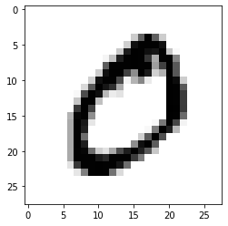
레이블 항목 출력하기
print(y_train[1])
/---------------/
# 출력
0
# index에 0에서 59999 사이 숫자를 지정.
index=10001
plt.imshow(x_train[index],cmap=plt.cm.binary)
plt.show()
print( (index+1), '번째 이미지의 숫자는 바로 ', y_train[index], '입니다.')
/--------------------------------------------------------------------/
# 출력
10002 번째 이미지의 숫자는 바로 8 입니다.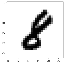
Matplotlib 이란?
파이썬에서 제공하는 시각화(Visualization) 패키지인 Matplotlib은 차트(chart), 플롯(plot) 등 다양한 형태로 데이터를 시각화할 수 있는 강력한 기능을 제공한다.
데이터셋 모양 확인하기
print(x_train.shape)
/------------------/
# 출력
(60000, 28, 28)print(x_test.shape)
/------------------/
# 출력
(10000, 28, 28)학습용 데이터, 검증용 데이터, 시험용 데이터?
교차검증이란?
데이터 전처리
이미지의 실제 픽셀 값은 0~255 사이의 값을 가진다.
print('최소값:',np.min(x_train), ' 최대값:',np.max(x_train))
/--------------------------------------------------------/
# 출력
최소값: 0  최대값: 255
인공지능 모델을 훈련시키고 사용할 때, 일반적으로 입력은 0~1 사이의 값으로 정규화 시켜주는 것이 좋다.
x_train_norm, x_test_norm = x_train / 255.0, x_test / 255.0
print('최소값:',np.min(x_train_norm), ' 최대값:',np.max(x_train_norm))
/------------------------------------------------------------------/
# 출력
최소값: 0.0  최대값: 1.0
딥러닝 네트워크 설계
텐서플로우 케라스(tf.keras)에서는 Sequential API라는 방법을 사용한다. Sequential API는 개발의 자유도는 많이 떨어지지만, 매우 간단하게 딥러닝 모델을 만들어낼 수 있는 방법이다.
그 밖에도 Functional API를 사용하는 방법도 있다.
model=keras.models.Sequential()
model.add(keras.layers.Conv2D(16, (3,3), activation='relu', input_shape=(28,28,1)))
model.add(keras.layers.MaxPool2D(2,2))
model.add(keras.layers.Conv2D(32, (3,3), activation='relu'))
model.add(keras.layers.MaxPooling2D((2,2)))
model.add(keras.layers.Flatten())
model.add(keras.layers.Dense(32, activation='relu'))
model.add(keras.layers.Dense(10, activation='softmax'))

print('Model에 추가된 Layer 개수: ', len(model.layers))
/---------------------------------------------------------------------------------/
# 출력
Model에 추가된 Layer 개수:  7
위 코드의 의미는 아래와 같다.
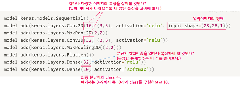
- Conv2D 레이어의 첫 번째 인자는 사용하는 이미지 특징의 수다. 여기서는 16과 32를 사용했다. 가장 먼저 16개의 이미지 특징을, 그 뒤에 32개의 이미지 특징씩을 고려하겠다는 뜻이다. 더 복잡한 영상이라면 특징 숫자를 늘려주는 것을 고려해 볼 수 있다.
- Dense 레이어의 첫 번째 인자는 분류기에 사용되는 뉴런의 숫자다. 이 값이 클수록 보다 복잡한 분류기를 만들 수 있다. 10개의 숫자가 아닌 알파벳을 구분하고 싶다면, 대문자 26개, 소문자 26개로 총 52개의 클래스를 분류해 내야 한다. 그래서 32보다 큰 64, 128 등을 고려해 볼 수 있을 것이다.
- 마지막 Dense 레이어의 뉴런 숫자는 결과적으로 분류해 내야 하는 클래스 수로 지정하면 된다. 숫자 인식기에서는 10, 알파벳 인식기에서는 52가 될 것이다.
모델을 확인하려면 model.summary() 메서드를 이용하면 된다.
model.summary()
/-------------/
# 출력
Model: "sequential_1"
_________________________________________________________________
Layer (type)                 Output Shape              Param #
=================================================================
conv2d_2 (Conv2D)            (None, 26, 26, 16)        160
_________________________________________________________________
max_pooling2d_2 (MaxPooling2 (None, 13, 13, 16)        0
_________________________________________________________________
conv2d_3 (Conv2D)            (None, 11, 11, 32)        4640
_________________________________________________________________
max_pooling2d_3 (MaxPooling2 (None, 5, 5, 32)          0
_________________________________________________________________
flatten_1 (Flatten)          (None, 800)               0
_________________________________________________________________
dense_2 (Dense)              (None, 32)                25632
_________________________________________________________________
dense_3 (Dense)              (None, 10)                330
=================================================================
Total params: 30,762
Trainable params: 30,762
Non-trainable params: 0
_________________________________________________________________
네트워크 학습하기
만들어 놓은 네트워크는 입력이 (데이터갯수, 이미지 크기 x, 이미지 크기 y, 채널수)와 같은 형태를 갖고 있다. 그런데 실제 데이터의 모양을 출력해보면 채널수에 대한 정보가 없다. 따라서 reshape()을 이용해 채널 수를 추가해준다.
print("Before Reshape - x_train_norm shape: {}".format(x_train_norm.shape))
print("Before Reshape - x_test_norm shape: {}".format(x_test_norm.shape))

x_train_reshaped=x_train_norm.reshape( -1, 28, 28, 1)  # 데이터갯수에 -1을 쓰면 reshape시 자동계산
x_test_reshaped=x_test_norm.reshape( -1, 28, 28, 1)

print("After Reshape - x_train_reshaped shape: {}".format(x_train_reshaped.shape))
print("After Reshape - x_test_reshaped shape: {}".format(x_test_reshaped.shape))
/-------------------------------------------------------------------------------------------/
# 출력
Before Reshape - x_train_norm shape: (60000, 28, 28)
Before Reshape - x_test_norm shape: (10000, 28, 28)
After Reshape - x_train_reshaped shape: (60000, 28, 28, 1)
After Reshape - x_test_reshaped shape: (10000, 28, 28, 1)
이제 실제 학습을 해보자. epoch 10은 10번 반복 학습 한다는 의미이다.
model.compile(optimizer='adam',
             loss='sparse_categorical_crossentropy',
             metrics=['accuracy'])

model.fit(x_train_reshaped, y_train, epochs=10)
/--------------------------------------------------/
# 출력
Epoch 1/10
1875/1875 [==============================] - 6s 3ms/step - loss: 0.1970 - accuracy: 0.9389
Epoch 2/10
1875/1875 [==============================] - 5s 3ms/step - loss: 0.0713 - accuracy: 0.9787
Epoch 3/10
1875/1875 [==============================] - 5s 3ms/step - loss: 0.0518 - accuracy: 0.9848
Epoch 4/10
1875/1875 [==============================] - 5s 3ms/step - loss: 0.0415 - accuracy: 0.9869
Epoch 5/10
1875/1875 [==============================] - 5s 3ms/step - loss: 0.0332 - accuracy: 0.9892
Epoch 6/10
1875/1875 [==============================] - 5s 3ms/step - loss: 0.0283 - accuracy: 0.9910
Epoch 7/10
1875/1875 [==============================] - 5s 3ms/step - loss: 0.0223 - accuracy: 0.9930
Epoch 8/10
1875/1875 [==============================] - 5s 3ms/step - loss: 0.0194 - accuracy: 0.9940
Epoch 9/10
1875/1875 [==============================] - 5s 3ms/step - loss: 0.0162 - accuracy: 0.9945
Epoch 10/10
1875/1875 [==============================] - 5s 3ms/step - loss: 0.0138 - accuracy: 0.9956
<keras.callbacks.History at 0x7fa850f4bf40>
각 학습이 진행됨에 따라 epoch 별로 어느 정도 인식 정확도(ccuracy)가 올라가는지 확인할 수 있다.
모델 성능 확인
모델 학습이 완료되었으니 테스트셋을 갖고 성능을 확인해보자.
test_loss, test_accuracy = model.evaluate(x_test_reshaped,y_test, verbose=2)
print("test_loss: {} ".format(test_loss))
print("test_accuracy: {}".format(test_accuracy))
/--------------------------------------------------------------------------/
# 출력
313/313 - 1s - loss: 0.0342 - accuracy: 0.9894
test_loss: 0.03419424220919609
test_accuracy: 0.9894000291824341
결과를 보면 99.57점을 받을 줄 알았는데, 98.85로 시험점수가 소폭 하락한 것을 확인할 수 있다. 즉, 한 번도 본 적이 없는 필체의 손글씨가 섞여 있을 가능성이 높다.
잘못 추론한 데이터를 직접 확인해보자.
model.evaluate() 대신 model.predict()를 사용하면 model이 입력값을 보고 실제로 추론한 확률분포를 출력할 수 있다. 확률값이 가장 높은 숫자가 바로 model이 추론한 숫자가 되는 것이다.
predicted_result = model.predict(x_test_reshaped)  # model이 추론한 확률값.
predicted_labels = np.argmax(predicted_result, axis=1)

idx=0  #1번째 x_test를 살펴보자.
print('model.predict() 결과 : ', predicted_result[idx])
print('model이 추론한 가장 가능성이 높은 결과 : ', predicted_labels[idx])
print('실제 데이터의 라벨 : ', y_test[idx])
/----------------------------------------------------------------------/
# 출력
model.predict() 결과 :  [6.0502055e-11 4.9696450e-07 5.3242346e-08 4.5255950e-09 1.4190464e-10
 4.1341784e-14 4.1637205e-17 9.9999940e-01 1.2403649e-08 2.1083607e-10]
model이 추론한 가장 가능성이 높은 결과 :  7
실제 데이터의 라벨 :  7
model.predict() 결과가 [6.0502055e-11 4.9696450e-07 5.3242346e-08 4.5255950e-09 1.4190464e-10 4.1341784e-14 4.1637205e-17 9.9999940e-01 1.2403649e-08 2.1083607e-10]와 같이 벡터형태로 나온다. 각 값은 0~9까지의 숫자일 확률을 의미한다.
해당 벡터값을 보면 model에서 추론하는 결과가 7일 확률이 1.00에 근접하고 있다. 즉, 이 모델은 숫자 7이라는 걸 아주 확신하고 있다는 뜻이 된다.
그럼 잘못된 데이터를 직접 출력해보자
import random
wrong_predict_list=[]
for i, _ in enumerate(predicted_labels):
    # i번째 test_labels과 y_test이 다른 경우만 모아보자.
    if predicted_labels[i] != y_test[i]:
        wrong_predict_list.append(i)

# wrong_predict_list 에서 랜덤하게 5개만 뽑아보자.
samples = random.choices(population=wrong_predict_list, k=5)

for n in samples:
    print("예측확률분포: " + str(predicted_result[n]))
    print("라벨: " + str(y_test[n]) + ", 예측결과: " + str(predicted_labels[n]))
    plt.imshow(x_test[n], cmap=plt.cm.binary)
    plt.show()
/----------------------------------------------------------------------------/
# 출력
예측확률분포: [6.9000855e-08 1.6199183e-05 1.5857623e-08 1.8698197e-06 1.1798908e-05
 4.9287152e-10 4.7909642e-13 5.5684513e-01 4.4309175e-01 3.3224554e-05]
라벨: 8, 예측결과: 7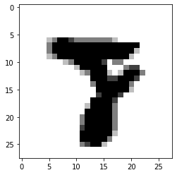
더 좋은 네트워크 만들기
# 바꿔 볼 수 있는 하이퍼파라미터들
n_channel_1=16
n_channel_2=32
n_dense=32
n_train_epoch=10

model=keras.models.Sequential()
model.add(keras.layers.Conv2D(n_channel_1, (3,3), activation='relu', input_shape=(28,28,1)))
model.add(keras.layers.MaxPool2D(2,2))
model.add(keras.layers.Conv2D(n_channel_2, (3,3), activation='relu'))
model.add(keras.layers.MaxPooling2D((2,2)))
model.add(keras.layers.Flatten())
model.add(keras.layers.Dense(n_dense, activation='relu'))
model.add(keras.layers.Dense(10, activation='softmax'))

model.summary()
model.compile(optimizer='adam',
             loss='sparse_categorical_crossentropy',
             metrics=['accuracy'])

# 모델 훈련
model.fit(x_train_reshaped, y_train, epochs=n_train_epoch)

# 모델 시험
test_loss, test_accuracy = model.evaluate(x_test_reshaped, y_test, verbose=2)
print("test_loss: {} ".format(test_loss))
print("test_accuracy: {}".format(test_accuracy))