The Fully Convolutional Transformer for Medical Image Segmentation(WACV, 2023)

박정민 (Jungmin Park)·2025년 2월 25일

논문 리뷰

목록 보기

17/21

1. Abstract

저자들은 의료 데이터에 대한 다양한 모달리티를 segmentation하는데 능한 transformer인 FCT를 제시하고 있습니다.
Fully Convolutional Transformer(FCT)는 잘 알려진 CNN으로 이미지의 표현을 배우고, Transformer로 이미지의 long term dependency들을 배우는 방식을 기반으로 모델링 됐습니다.
FCT는 먼저, long range semantic dependency를 배우고, 계층적 global함을 배우는 단계, 총 2개의 단계로 input을 처리합니다.

2. Introduction

현대의 image segmentation model들은 주로 top-down(encoder-decoder) 구조로 입력 이미지를 압축하여 latent 공간에 넣고, 그 다음에 관심 지역들을 decode하는 방식을 채택합니다. 여기에 skip connection을 횡방향으로 연결해주어서 image segmentation 분야에서 큰 도약을 하게 해준 UNet의 구조를 가지게 합니다.
UNet의 키포인트는 fully convolutional하며, non-convolutional 한 parameter들은 예측하지 않는다는 점에 있습니다.
하지만, UNet은 지역적인 부분밖에 볼수 없어(CNN의 단점) global dependency를 보게 해줌으로써 발전을 시키려고 하는 노력들을 해왔습니다. 이에는 attention을 추가한다던지, kernel size를 키워서 볼 수 있는 영역을 넓히는 방식 등이 있지만, 각 방법에는 각자의 단점이 존재합니다.
Transformer는 자연어 처리에서 큰 성공을 거두었고, ViT로 인해서 이미지 task에도 접목이 되면서, ViT를 발전시켜서 Swin transformer와 같이 방대한 데이터나 계산량 없이도 가능하다는 것을 보였습니다.
ViT 계열의 transformer들은 서로 겹치지 않는 패치로 이미지를 나누고, spatial한 위치 정보를 positional encoding 해주어서 패치들과 같이 transformer 레이어들에 통과시켜 long range dependency를 학습할 수 있도록 합니다.
이 둘의 장점만을 취하기 위해서 최근에는 CNN-Transformer을 섞은 hybrid model들이 많이 등장하고 있는데, 이 다음 단계는 CNN만으로 두 장점을 모두 취할 수 있게 설계하는 것이라고 생각해서 fully convolutional한 모델을 소개하고 있습니다.

3. Fully Convolutional Transformer

Dataset이 {X, Y}로 이루어졌다고 가정했을 때, X는 입력 이미지, Y는 이에 대해 segmentation되어 있는 semantic or binary segmentation map이라고 합니다.
입력 이미지는 3D 이미지를 slicing해서 얻은 (H, W, C) 차원을 가지는 2D 이미지여야 하고, 출력으로는 (H, W, D) 차원을 가지는 segmentation map이 나옵니다. (단, 여기서 D는 클래스 개수)
본 논문의 방법은 cnn-transformer hybrid도 아니며, 사전 학습을 하고 온 transformer를 사용하는 Unet 구조도 아니라는 점에서 이전의 연구들과는 다르다고 합니다.
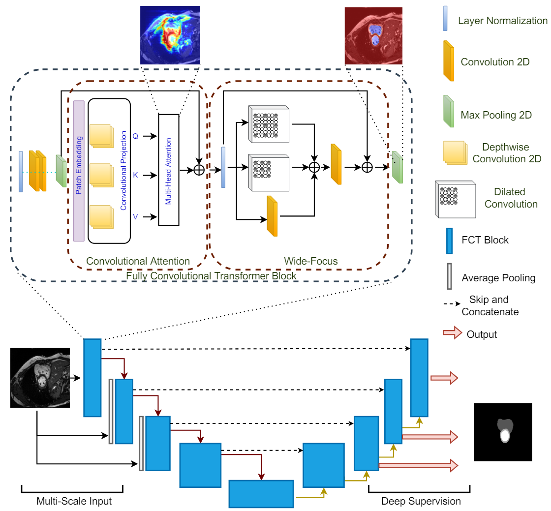
FCT Block은 먼저 겹치는 patch들을 이미지에서 추출하고, patch 기반 임베딩을 생성하여서 multi-head-self-attention을 patch들에 적용합니다.
주어진 이미지들의 output projection은 Wide-Focus라는 모듈로 전달되어 fine한 정보를 추출하게 됩니다.

4. FCT layer

각 FCT layer는 LayerNorm-Conv-Gelu-Conv-Gelu-Maxpool 연산으로 시작된다. 이 이유는 3x3 convolution을 패치들에 sequent하게 적용하는 것이 바로 patch-wise projection을 하는 것보다 인코딩이 잘된다고 합니다.
Maxpool의 출력은 Depthwise convolution 연산인 T(.) 으로 들어가게 된다. 커널 크기는 3x3이며, stride는 s x s인데, 여기서 기존과 다른 점은 1. 추출된 패치들은 서로 겹치는 패치이다. 2. Depthwise 컨볼루젼 연산이 출력의 크기를 변화시키지 않는다 로 총 2가지 입니다. 즉, 모든 패치들은 인풋 이미지와 사이즈가 동일합니다.
이후에 Layer Normalization을 통과하게 되고 token map을 얻게 되면 이는 WH x C의 차원을 가지는 patch embedded input이 됩니다.
대부분의 model들은 Multi-Head self attention을 위해 linear projection을 채택하며 이로 인해 spatial한 정보에서 손실이 생기기 마련인데, 이를 보완하기 위해 convolution layer를 추가하지만 이는 계산량을 증가시킨다는 문제가 있습니다.
이를 해결하기 위해 본 논문에서는 MHSA block안에 linear projection을 Depthwise Convolution으로 대신하여 계산량을 줄이면서도 spatial한 정보의 손실을 줄입니다. 이렇게 Convolutional Attention은 patch embedding과 convolutional attention projection으로 이루어져 있습니다.
논문의 경우에는 Batch Normalization을 Layer Normalization으로 대체하는 것이 더 좋은 성능을 보였으며, Point-wise convolution은 제거하는 것이 성능 손실 없이 모델을 더욱 간결하게 만들어주었다고 합니다.
이렇게 Depthwise Convolution으로 positional encoding의 필요성을 삭제하면서 더욱 더 간결한 모델의 구조를 얻었다고 합니다.
또한, MHSA 연산 뒤에 주로 쓰이는 linear layer를 convolution layer로 대체하는 것은 spatial한 context를 잃는 것을 방지하기에, 성능의 큰 향상을 가져온다고 합니다.
하지만, 의료 분야에서는 이에 더해서 fine한 정보 처리를 요구하기 때문에 저자들은 한 쪽에서는 그냥 convolution을 하고, 병렬적으로 동시에 dilated convolution을 실행하여 spatial한 context를 더 잘 추출해내는 multi-branch convlolution layer를 채택합니다.
이 후에 output feature를 summation하여 합친 후 convolution layer를 통과시킵니다. 이러한 과정을 모두 합쳐 Wide-focus라는 모듈이라고 부른다. 중간 중간 residual connection으로 성능을 향상시켰고, 연산된 feature는 다음 FCT layer로 넘겨집니다.

5. Encoder

총 4개의 FCT layer로 이루어져 있으며, l번째 transformer layer에 대해서 Convolutional Attention module의 출력은
$z_l' = MHSA(z_l) + z_{l-1}^{q/k/v}$ ,
$z_{l-1}^{q/k/v} = Flatten(DepthConv(Reshape(z_{l-1})))$ .
MHSA는 $MHSA(z_{l-1}) = softmax(\frac{QK^T}{\sqrt{d}})V$ 의 식을 가집니다.
위의 방식으로 계산된 $z'_l$ 은 Wide-focus module에서 $z_l = WF(z_l) + z'_l$ 식에 의해 계산됩니다.
이에 더해 encoder에 pyramid style로 다양한 scale에서의 인풋을 넣어주어서 여러 scale에서도 multi-class 혹은 작은 물체도 segmentation 할 수 있도록 만들지만, 이러한 작용 없이도 SOTA를 달성한다고 합니다.
bottleneck encoding은 그냥 또 다른 하나의 FCT layer를 사용하여 수행한다고 합니다.

6. Decoder

Decoder는 bottleneck으로 부터 input으로 받은 표현을 segmentation map을 re-sample하는 역할을 합니다.
U-net과 동일하게 조금 더 정보를 잘 받기 위해서 encoder 부분에서 skip connection으로 feature map들을 받아옵니다.
decoder의 구조는 encoder와 비슷합니다.
낮은 해상도에서는 deep supervision을 사용하였고, 가장 낮은 해상도인 28 x 28에서는 사용하지 않았다고 합니다. 이유는 ROI 영역 즉, segmentation되어있는 부분이 때때로 너무 작아서 segmentation이 검출되지 않는 경우가 있어서 worst한 모델 성능을 보였기 때문입니다.

7. Experiments

ACDC dataset과 ISIC 2017에 대해서는 7:1:2으로, Spleen dataset(CT)는 8:1:1로 split하였고, 모든 성능 평가는 dice coefficient를 사용하였다고 합니다.
모든 실험은 tensorflow 2.0에서 1개의 A6000 GPU로 진행되었으며, loss function은 Cross Entropy Loss와 Dice Loss 2가지를 5:5로 동일하게 weighting하여 사용했다고 합니다.
Optimizer은 Adam Optimizer를 사용하였고, lr은 1e-3로 시작하여 validation loss를 따라서 감소하도록 하였다고 합니다.
warmup epoch은 50으로 설정하였고, 추후에 250epoch더 진행하여 총 300epoch의 학습을 했다고 합니다.
Data Augmentation 기법으로는 rotation, shear, zoom, horizontal/vertical shift & flip을 사용하였다고 합니다.
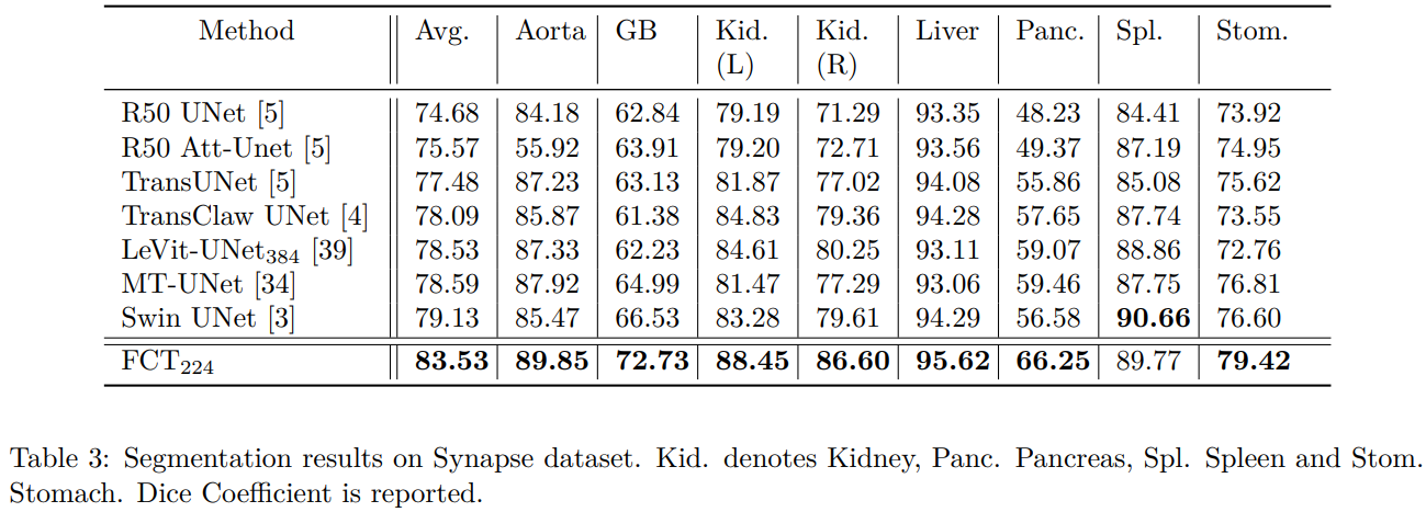
기존의 연구중 가장 가까운 경쟁 상대인 nnFormer보다 5배 작은 모델 사이즈로 SOTA를 달성했다고 합니다.
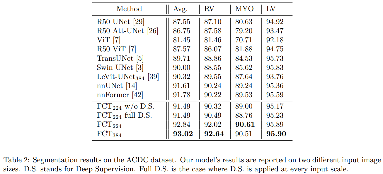
학습은 384x384와 224x224 2 가지를 진행했다고 하며 384의 경우가 확실히 fine한 spatial 정보를 더 잘 볼 수 있어서 성능이 좋았다고 합니다.
별도로 deep supervision을 모든 스케일에서 사용하는 것과 그렇지 않은 것을 실험했는데, 논문에서 제시하는 방식이 최고의 성능을 보인다고 합니다.

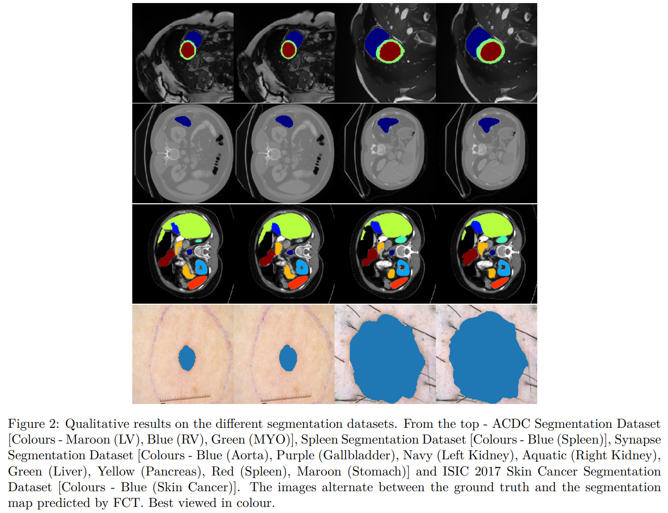
Qualitative Results on ACDC/Spleen/Synapse/ISIC2017

Quantitative Results on ACDC Dataset

Quantitative Results on Synapse Dataset

8. Ablation Study

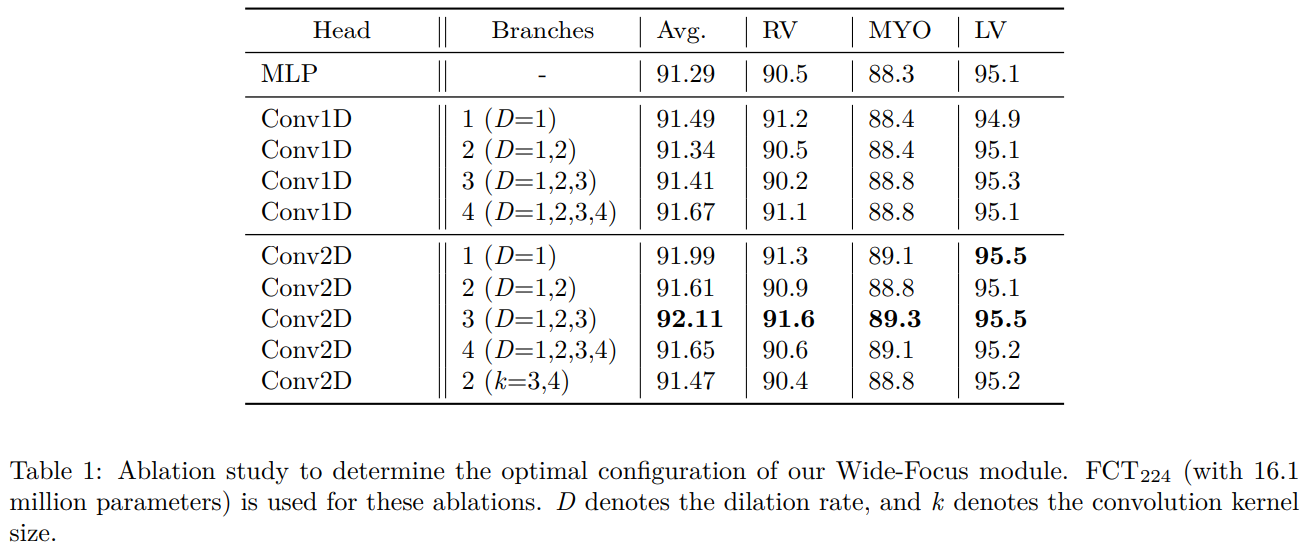
Ablation Study로는 skip connection을 제거하는 것과, wide focus module에서의 dilate convolution의 병렬적인 개수를 늘리는 실험을 해보았는데, skip connection은 performance에 매우 중요한 영향을 끼치고 있었고, dilate convolution을 늘리는 것은 3개의 branch 이상으로 가면 성능이 점점 포화되다가 결국 감소하는 경향을 보였다고 합니다.

Ablation of Wide-Focus Module

9. Conclusion

FCT는 기존의 모델과 비교하였을 때, 3-5배 적은 모델 파라미터로 SOTA를 달성한다고 합니다.
본 논문에서는 2가지 key point를 제시하고 있는데, Convolutional Attention과 Wide-Focus입니다.
Convolutional Attention에서는 linear projection을 depthwise convolution으로 대체하여 겹치는 patch들을 생성하며 positional encoding의 필요성을 제거하여 연산량을 줄이고, 성능을 유지하였습니다.
Wide Focus Module에서는 일반적은 conv layer와 더불어서 dilated convolution을 함께 사용하여 add하는 방식으로 작고 fine한 정보를 잘 배워 성능을 향상시켰다고 합니다.
FCT Block은 medical image application에서 최초로 fully convolutional한 transformer block이며, 손쉽게 다른 medical domain이나 application에 적용될 수 있다고 합니다.

10. English Summary

This paper is proposing ‘The Fully Convolutional Transformer’ which is capable of accurately performing binary and semantic segmentation tasks with over 3-5 times fewer parameters than existing models.
The FCT Layer starts with Layer Normalization-Convolution-Convolution-Maxpool and each Convolution is Followed by a GeLU activation layer.
Applying consecutive convolution layers with small kernels was more effective then directly creating patch-wise projections.
The FCT Layer comprises of two key components - Convolutional Attetntion and Wide-Focus
Convolutional Attention removes the need for positional encoding at the patch creation stage by using Depthwise-Convolutions to create overlapping patches for the model. This makes the model architecture more simple.
The 2 differences from existing researches are that they use overlapping patches which have the same spatial size as the input image.
They also use Depthwise-Convolution based MHSA block, which integrates spatial information to estimate long range semantic dependencies for the first time in a medical imaging context.
Their Wide Focus Module helps leverage fine-grained feature information present in medical images and is an important factor in boosting the performance of their transformer block
Multi Branch Convolution is used in the Wide Focus model to extract better fine-grained information.
The Encoder Part is composed of 4 FCT Layers in total, and multi-scaled inputs can be used to enhance performance for small objects.
The Decoder Part learns to re-sample the segmentation maps from the latent representation input.
Also, skip connections are used to get feature information from the Encoder Part for better performance.
Deep supervision was used in low resolutions except for the lowest resolution, because often the ROIs in the input image scans were too small to segment at the lowest scale. It is said that this low scale output added a strong bias in the model to predict some output ROIs as the background class.