[Paper Review] Transformers are RNNs: Fast Autoregressive Transformers with Linear Attention

Summary

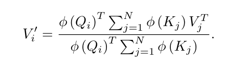
• If the similarity in attention is expressed as a kernel $\phi(Q_i)^T\phi(K_j)$ using a feature map $\phi$, $\phi(Q_i)$ can be separated out of the sum over $j$. Then $\sum_j \phi(K_j)V_j^T$ and $\sum_j \phi(K_j)$ can be computed only once and reused by every query, so the computation time and memory become $O(N)$.

• With causal masking, it is enough to carry $\sum_{j \le i}\phi(K_j)V_j^T$ as a cumulative sum (state), which means that a Transformer layer = an RNN with a fixed-size hidden state.

• As a result, autoregressive generation runs inference with constant time and constant memory per step without a KV cache, and is about 4,462 times faster than softmax on CIFAR-10 image generation.

1. Problem & Motivation

Transformers have shown strong performance on a variety of tasks including natural language, and pre-training with autoregressive / masked LM objectives yields powerful representations even from unlabeled data. However, since self-attention computes the similarity of every key-query pair, for an input of length $N$ it has time complexity $O(N^2)$ and memory $O(N^2)$, which limits the context length. In particular, in autoregressive inference, attention is applied over all tokens so far every time a single token is generated, so the per-step cost keeps growing as generation gets longer.

To reduce the existing time complexity and memory, this paper introduces the Linear transformer architecture.

Linear Transformer computes similarity with a kernel-based formulation so that both memory and computation become $O(N)$.

2. Related Work

2.1. Efficient Transformers

Several methods have previously been proposed to speed up training and inference. Weight pruning, factorization, quantization, etc. speed up training and inference, but the time complexity of the attention operation is still $O(N^2)$.

Attempts to increase context by reducing complexity are as follows. Both methods*reduce complexity by having each query look at only a subset of keys.

• Sparse Transformer (Child et al.): factorizes the attention matrix sparsely so that each query only looks at positions in a fixed pattern, with complexity $O(N\sqrt{N})$.
• Reformer: puts similar vectors into the same bucket and computes attention only within a bucket. Hashing requires the constraint $Q = K$, and the complexity is $O(N\log N)$.

Context is the maximum range of the sequence that can be used when computing self-attention. In $O(N^2)$ attention, as the sequence gets longer, the amount of computation and the memory for storing the attention matrix grow quadratically, which limits the context length. Reducing complexity allows longer sequences to be processed with the same resources, so reducing complexity can ultimately be seen as a way to handle long sequences.

Unlike previous methods, Linear Transformer scales linearly with sequence length without any constraints on queries and keys.

2.2. Understanding Self-Attention

From a kernel perspective, attention can be thought of as applying to the input a kernel smoother, which takes an average giving higher weights to more similar data. Here, the kernel value is the similarity between inputs.

This paper extends the above perspective and applies the idea that any kernel giving positive similarity scores can be used as attention. Additionally, it shows that a self-attention layer trained with an autoregressive objective can be viewed as an RNN.

3. Linear Transformers

3.1. Transformers

The input $x \in \mathbb{R}^{N \times F}$ is a sequence of $N$ feature vectors of dimension $F$. A Transformer layer $T_l$ consists of self-attention $A_l$ and a feedforward $f_l$.

Here $Q = xW_Q$, $K = xW_K$, $V = xW_V$. The $i$-th output of softmax attention can be generalized using a similarity function $\text{sim}(\cdot,\cdot)$.

If $\text{sim}(q, k) = \exp\left(\frac{q^Tk}{\sqrt{D}}\right)$, it becomes the standard softmax attention. That is, as long as $\text{sim}$ is non-negative, any function can be used as attention.

3.2. Linearized Attention

If the kernel $k(x, y): \mathbb{R}^{2 \times F} \to \mathbb{R}_+$ is expressed with a feature map $\phi$ so that $\text{sim}(Q_i, K_j) = \phi(Q_i)^T\phi(K_j)$,

Since $\phi(Q_i)$ is independent of $j$, it can be pulled out of the sum. Because $Q_i$ can be separated, the computation for $Q_i$ can be done only once.

• The original approach builds the $N \times N$ matrix first → $O(N^2)$
• The approach with $Q_I$ pulled out builds $\phi(K)^TV$ (a $D \times M$ matrix) first → $O(N)$

Since $\sum_{j}\phi(K_j)V_j^T$ and $\sum_{j}\phi(K_j)$ are computed only once and reused by every query, time and memory become linear in $N$.

3.3. Feature Maps and Computational Cost

This paper chose the following feature map.

The function $\phi(x)=elu(x)+1$ has the following properties

• Thanks to the $+1$, $\phi(x) > 0$, so the similarity is always positive
• It prevents the gradient from becoming 0 when $x$ is negative.

3.4. Causal Masking

In an autoregressive model that generates one token at a time, the $i$-th position must only be influenced by positions with $j \le i$. To apply causal masking to the linearized attention expressed as in $3.2.$, only the range of the sum needs to change from $N$ to $i$.

Here, the terms grouped by $\sum$ are sums from the first to the $i$-th position, growing by one term as $i$ increases. That is, instead of computing from $i=1$ every time, it can be thought of as a cumulative sum where one value is added for each new position $i$.

If the cumulative sums are defined as follows

and they are updated from the previous values in constant time as $S_i = S_{i-1} + \phi(K_i)V_i^T$, $Z_i = Z_{i-1} + \phi(K_i)$. Therefore, the entire causal attention is linear in sequence length.

3.5. Gradient Computation

If all $S_i$ were stored and differentiated with autograd, memory would become $O(NDM)$, possibly using even more memory than softmax. Therefore, the paper solves this by expressing the gradients themselves as cumulative sums as well.

In this way, both forward and backward can be processed in linear time and memory.

3.6. Transformers and RNNs

The key idea of interpreting linear attention as an RNN is as follows.

Any Transformer layer with causal masking can be written as a model that takes an input, updates an internal state, and produces an output, i.e., an RNN.

• Hidden state: $s_i \in \mathbb{R}^{D \times M}$ (attention memory), $z_i \in \mathbb{R}^{D}$ (normalizer memory)
• When a new token $x_i$ comes in, the state is updated, and the output is produced by reading the state with the current query.
• During training it can be used like a Transformer that processes all positions in parallel, and during inference like an RNN that carries only the state.

A softmax Transformer must store all past tokens' K and V in the KV cache, so the cost per generation step grows as $O(N)$, whereas a Linear Transformer only needs to maintain a single fixed-size state, so the per-step cost and memory are constant.

4. Experiments

4.1. Setup

The three compared methods are as follows.

• Softmax: standard full attention Transformer
• LSH-X: Reformer. X is the number of hashing rounds
• Linear: Linear Transformer using $\phi(x) = \text{elu}(x) + 1$

The experiments cover a synthetic task, image generation (MNIST, CIFAR-10), and more.

4.2. Synthetic Task: Convergence

Convergence behavior was compared on a copy task (copying a sequence of symbols as is), similar to sequence duplication.

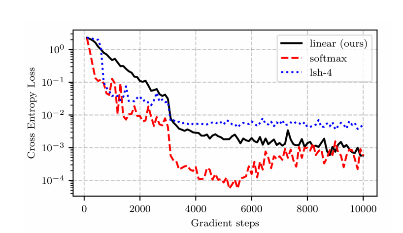
• Linear converges stably (smoothly) and reaches a lower loss than LSH-4.
• It eventually reaches a loss similar to softmax. However, in the middle range (about 4,000–7,000 steps), softmax shows a lower loss.

4.3. Synthetic Task: Memory & Computation

GPU peak memory and forward/backward time were measured while varying the sequence length from $2^9$ to $2^{16}$.

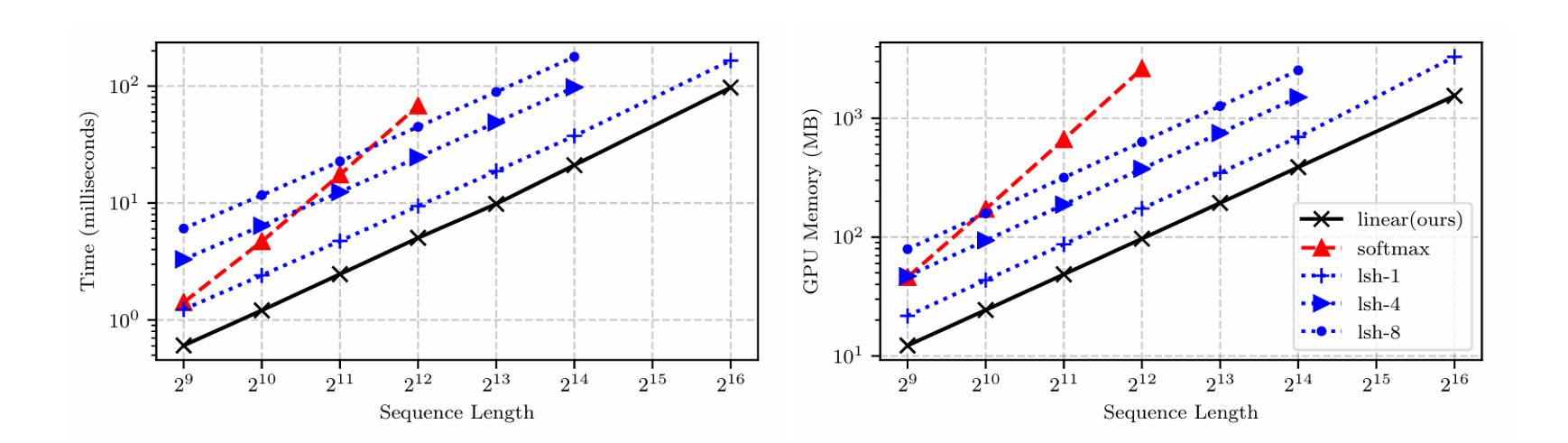
• Softmax grows quadratically with length and cannot be measured beyond $2^{12}$ (out of GPU memory).
• Both LSH and Linear grow linearly, but Linear is the fastest and uses the least memory at every length.

4.4. Image Generation: MNIST & CIFAR-10

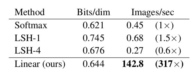
Images are generated autoregressively pixel by pixel. The evaluation metrics are bits/dim (lower is better) and the number of images generated per second.

MNIST

CIFAR-10

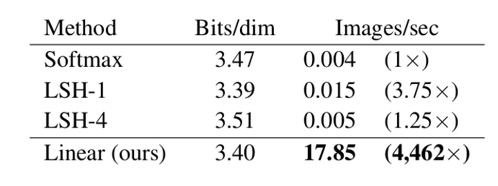
• Linear achieves quality similar to softmax while generating 317 times faster on MNIST and 4,462 times faster on CIFAR-10. That is, while softmax generates a single CIFAR-10 image, Linear generates about 4,460 images.
• The speed gap becomes much larger on CIFAR-10, which has longer sequences. This is because softmax's cost grows every step, while Linear's per-step cost stays constant like an RNN.

5. Conclusion

Linear Transformer replaces attention with an inner product of kernel feature maps and uses the associativity of matrix multiplication to reduce time and memory complexity from $O(N^2)$ to $O(N)$. In addition, by interpreting causal attention as an RNN, it enables autoregressive inference with constant time and constant memory. In experiments, it maintained performance close to softmax while achieving speedups of hundreds to thousands of times in autoregressive generation.

6. My Take

1. An optimization in a different direction from MQA → GQA → MLA
MQA, GQA, and MLA, which I have read so far, were all answers to "how small can the KV cache be stored?" Whether heads are shared (MQA, GQA) or compressed into a latent (MLA), the cache still grows in proportion to the number of tokens $N$. Linear Transformer discards per-token K and V of past tokens altogether and summarizes them into a single state of size $D \times M$. It is a fundamentally different approach in that the KV cache size becomes independent of $N$.

2. Compressing the entire past into a fixed-size state
Softmax attention keeps all past tokens and can retrieve exactly what it needs. In contrast, Linear attention's $S_i$ simply adds up all $\phi(K_j)V_j^T$, so as the length grows, information gets mixed and it becomes hard to accurately recover a specific token. I think the much lower loss of softmax in the middle range of the copy task and the slightly worse MNIST bits/dim can also be seen in connection with this limitation.

References

• Katharopoulos, A., Vyas, A., Pappas, N., & Fleuret, F. (2020). Transformers are RNNs: Fast Autoregressive Transformers with Linear Attention. ICML 2020. arXiv:2006.16236
• Vaswani, A. et al. (2017). Attention Is All You Need. arXiv:1706.03762
• Child, R. et al. (2019). Generating Long Sequences with Sparse Transformers. arXiv:1904.10509

This post was translated from the original Korean version with the help of AI, so some errors may remain.