[Paper review] DeepSeek-V2: A Strong, Economical, and Efficient Mixture-of-Experts Language Model
Paper review
Summary
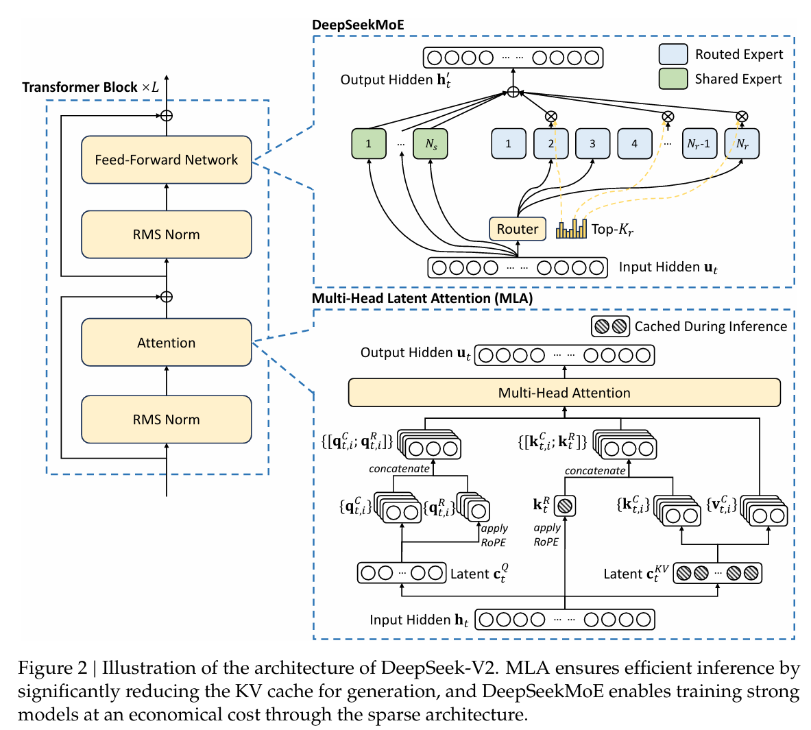
- MLA (Multi-head Latent Attention): Keys and values are jointly compressed into a single low-dimensional latent vector, and only this latent is cached. The KV cache shrinks to the level of GQA, yet performance is actually better than MHA.
- DeepSeekMoE: Instead of every token sharing all experts in the FFN layer, the model uses a few shared experts plus routed experts selected by affinity scores. On top of this, device-limited routing and three balance losses reduce the communication cost of expert parallelism.
- Effect: Out of 236B total parameters, only 21B are activated per token. Compared with DeepSeek 67B, training cost drops by 42.5%, the KV cache shrinks by 93.3%, and maximum generation throughput increases 5.76×.
1. Problem & Motivation
As LLMs grow in parameter count, emergent capabilities appear and performance improves. The price is a larger training compute budget, and at inference time, generating each token requires caching the keys and values of all previous tokens. This KV cache consumes memory capacity and memory bandwidth, which in turn lowers throughput.
GQA and MQA are the standard existing remedies. They reduce the cache by having multiple attention heads share the same keys and values, either in groups (GQA) or all together (MQA). Because heads share K and V, however, both perform worse than MHA. To address this, DeepSeek-V2 proposes two techniques.
- Multi-head Latent Attention: An attention mechanism equipped with low-rank key-value joint compression
- DeepSeekMoE: Fine-grained experts with shared expert isolation
2. Core Idea ①: Multi-head Latent Attention (MLA)
2.1 Low-Rank Key-Value Joint Compression
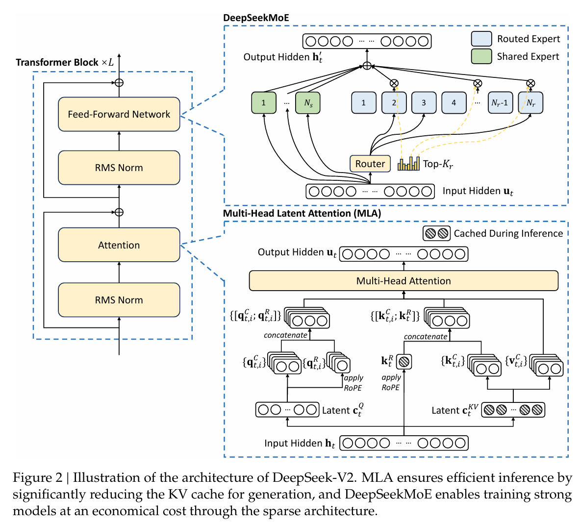
The core idea of low-rank key-value joint compression is to avoid caching K and V directly. Instead, the model caches only a latent vector from which K and V can be reconstructed.
The token embedding is compressed into . At inference time only is cached, and and are recovered through and .
- : input hidden state of the -th token
- : down-projection that compresses the input into , where
- : up-projections that reconstruct each head's K and V from the latent
Since only is cached at inference, each token needs just elements per layer, far fewer than the elements required by standard MHA. In practice, K and V are not even recomputed at every step. Because is multiplied with the query and is multiplied with , can be absorbed into the query projection and into . As a result, attention can be computed directly on the latent without explicitly reconstructing K and V.
In this way, low-rank key-value joint compression reduces memory access at the cost of more GPU computation. Is trading memory access for extra computation actually worthwhile?
The latency for a GPU to process one step can be expressed as follows.
- : amount of data read from and written to memory (bytes)
- : memory bandwidth (bytes/s)
- : number of floating-point operations (FLOPs)
- : peak compute throughput of the GPU (FLOP/s)
During decoding, attention consists of simple multiply-add operations within matrix multiplications, so the workload is memory-bound. Increasing the FLOP count therefore does not increase . In other words, it is far more effective to reduce at the cost of a larger .
2.2 Query Compression: Saving Activation Memory
Queries are compressed into a low-dimensional latent in the same way.
Queries are not cached, so this compression is not for inference. Its purpose is to reduce activation memory during training, that is, the intermediate values that must be stored for backpropagation.
2.3 Decoupled RoPE
RoPE multiplies keys by a position-dependent rotation matrix, which inserts a position-dependent matrix between and the query. As a result, can no longer be pre-absorbed into , and the keys of all past tokens would have to be reconstructed at every inference step, eliminating the benefit of MLA.
To solve this, MLA separates the part of the query and key responsible for positional information.
- The RoPE-applied query is kept per head, while the RoPE-applied key is shared across all heads.
- The cached quantities are and , totaling elements per token.
- With the RoPE and non-RoPE parts separated, the dot product splits into multiplied with and multiplied with . The latter still allows to be absorbed. Meanwhile, is not reconstructed from the latent; it is computed directly from and cached with RoPE already applied. Consequently, no key reconstruction is needed at all.
2.4 KV Cache Comparison
| Attention | KV cache per token (# elements) | Capability |
|---|---|---|
| MHA | Strong | |
| GQA | Moderate | |
| MQA | Weak | |
| MLA | Stronger |
DeepSeek-V2 sets and . As a result, the MLA cache is the same size as GQA with only 2.25 groups, while performance exceeds MHA. This is the paper's most important result.
3. Core Idea ②: DeepSeekMoE
3.1 Basic Structure
DeepSeekMoE consists of two main ideas.
Fine-grained expert segmentation: Each expert, an FFN obtained by splitting the original FFN into several pieces, is made smaller, and many of them are activated at once. The rationale is that the larger number of possible expert combinations allows the model to learn more diverse features.
Shared expert isolation: In addition to the experts activated differently for each token, shared experts that every token always passes through are introduced to capture common knowledge. This aims to reduce redundant knowledge learned across routed experts.
Each layer of DeepSeek-V2 has 2 shared experts and 160 routed experts, and 6 routed experts are activated per token.
3.2 Device-Limited Routing
Under expert parallelism, experts are distributed across multiple GPUs. The more devices a token's selected experts are spread over, the higher the communication cost, since communication frequency is proportional to the number of devices covered by the target experts.
Routing is therefore split into two stages. The model first selects the devices holding the experts with the highest affinity scores, and then performs top-K selection only among the experts on those devices. The paper reports that achieves performance comparable to unrestricted routing.
3.3 Auxiliary Losses for Load Balance
Three balance losses are used to prevent tokens from concentrating on particular experts or GPUs.
1) Expert-level balance loss: prevents imbalance among experts.
- is how often expert is actually selected, and is the average affinity score of expert .
2) Device-level balance loss: prevents imbalance in computation across devices.
3) Communication balance loss: balances the number of tokens each device receives, since device-limited routing only bounds communication on the sending side.
Although the three losses target different things, they all share the same form. Each represents the actual selection ratio relative to the case where devices or experts are chosen uniformly, and the resulting losses encourage all devices and experts to be selected evenly.
3.4 Token-Dropping Strategy
Balance losses alone cannot guarantee strict load balance. During training, a device-level token-dropping strategy is therefore applied. A computational budget (capacity) is set for each device, and when it is exceeded, tokens with the lowest affinity scores are dropped first. To reduce the mismatch between training and inference, about 10% of the sequences are never dropped.
4. Pre-Training
4.1 Setup
- Data: High-quality data from diverse sources was added, with quality-based filtering and bias removal. The model was trained on 8.1T tokens in total.
- Model: 60 layers, , , . Out of 236B total parameters, 21B are activated per token.
- Training: AdamW with a warmup-and-step-decay schedule. Training used DeepSeek's in-house HAI-LLM framework, and thanks to the small number of activated parameters, the model could be trained without tensor parallelism.
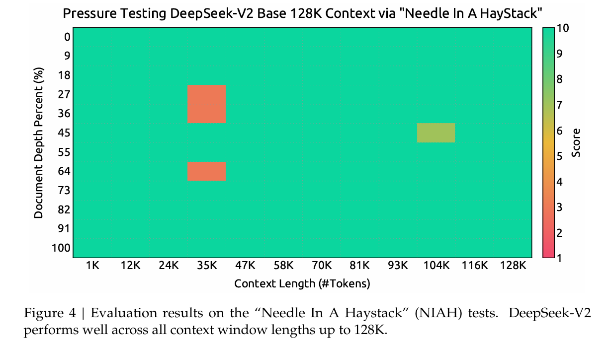
- Long context: YaRN was applied to the decoupled key to extend the context window from 4K to 128K. Long-context capability was verified with the Needle In A Haystack test.
4.2 Evaluation
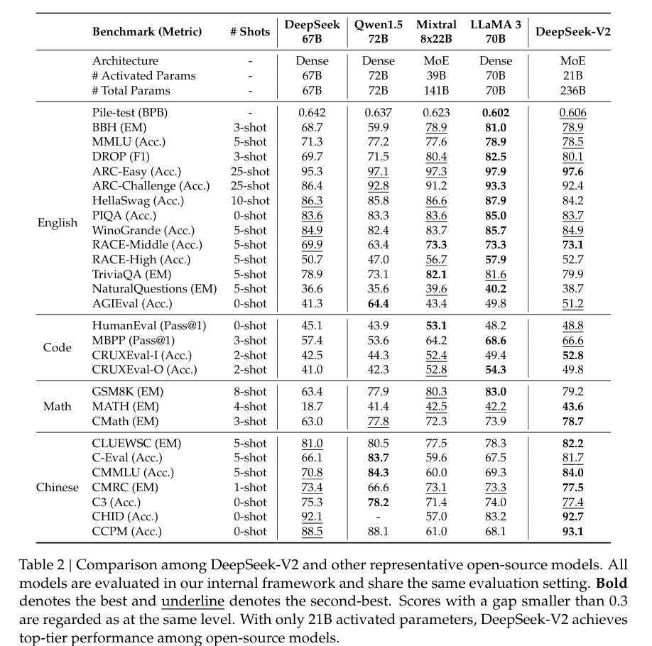
- DeepSeek-V2 outperforms DeepSeek 67B on almost all benchmarks and ranked among the top open-source models at the time of release.
- Training costs: 172.8K GPU hours per trillion tokens, 42.5% less than DeepSeek 67B (300.6K).
- Inference efficiency: The KV cache is quantized to an average of 6 bits per element, and the smaller cache allows serving with larger batch sizes. As a result, maximum generation throughput increased 5.76×.
5. Alignment
5.1 SFT (Supervised Fine-Tuning)
1.5M instruction instances were used: 1.2M for helpfulness and 0.3M for safety. Data quality was improved to reduce hallucinated responses and strengthen writing ability.
5.2 Reinforcement Learning: GRPO
In conventional RL, computing the advantage requires training an additional critic model to estimate the baseline. Since the critic is typically about the same size as the policy, this hurts training efficiency. GRPO removes the critic and instead estimates the baseline from the reward statistics of outputs sampled for the same question.
Training proceeds in two stages.
- Reasoning alignment: Trained on code and math reasoning tasks with .
- Human preference alignment: Combines multiple rewards:
For training efficiency, a hybrid engine that adopts different parallelism strategies for training and inference was introduced, and large batch sizes were used to speed up inference sampling.
5.3 Evaluation Results
- Base → SFT: Math and code performance improved substantially because of their large share in the SFT data.
- SFT → RL: Further gains were observed on reasoning-related tasks, especially math and code generation.
- Amount of SFT data: Prior work suggested that around 10K instances are sufficient. In DeepSeek-V2, however, reducing the data degraded instruction-following ability. The interpretation is that acquiring a given capability requires a minimum amount of data, and that amount does not approach zero.
6. My Take
6.1 Why does MLA outperform MHA?
MLA does not produce K and V directly; it compresses them once and then reconstructs them. The structure inevitably loses information, yet MLA outperformed MHA on many tasks in the experiments. What I was most curious about was why. (At inference time, weight absorption removes the explicit reconstruction step, but the representational bottleneck remains the same.)
I came up with two possible explanations.
- Contribution of the query? In KV-sharing methods such as GQA, the diversity of queries may matter more for performance than that of K/V. However, MLA compresses the query as well, so the query is unlikely to be the cause.
- The shared latent as a regularizer? Compressing K and V into a single common vector may lead the model to learn more generalized representations. Projecting into a low-rank space keeps only the most important features.
Of the two, I find the second more plausible, but the paper includes no ablation that directly tests this, so the exact cause remains an open question. Varying and observing the change in performance could help verify this hypothesis to some extent. I also suspect that for tasks with longer contexts and much more data and samples, MHA might still achieve better raw performance when GPU efficiency is not a concern.
6.2 Why is splitting experts into finer pieces beneficial?
DeepSeekMoE uses far more, smaller experts than conventional MoE and activates many of them at once. But if the total number of parameters and the activation ratio are the same, I wondered why there should be any theoretical difference in expressiveness between splitting experts finely and keeping them large.
- The number of combinations certainly increases, but does each expert really learn a separate sub-skill? Common information could also be learned across routed experts, and since humans cannot directly inspect this, I wondered whether sub-skills are actually learned in a separated way.
- If some experts have overlapping roles, is there a way to distinguish or measure them?
- Also, if the purpose of separating experts is for shared experts to learn common features and routed experts to learn finer-grained ones, would giving the experts different sizes make the features each one learns more clearly distinguishable?
6.3 Are shared experts really necessary?
I wondered whether common knowledge could be learned through routing alone, without shared experts. From the outside, it is impossible to tell which skill each expert is responsible for. An expert that has learned common knowledge might then naturally receive high affinity scores for every token and effectively behave like a shared expert. In that case, however, the balance losses would work to suppress such concentration. So it may be more accurate to view shared experts as a mechanism that resolves the conflict between the balance losses and the learning of common knowledge.
References
- DeepSeek-AI. DeepSeek-V2: A Strong, Economical, and Efficient Mixture-of-Experts Language Model. arXiv:2405.04434, 2024.
- Dai et al. DeepSeekMoE: Towards Ultimate Expert Specialization in Mixture-of-Experts Language Models. arXiv:2401.06066, 2024.
- Shao et al. DeepSeekMath: Pushing the Limits of Mathematical Reasoning in Open Language Models (GRPO). arXiv:2402.03300, 2024.
- Ainslie et al. GQA: Training Generalized Multi-Query Transformer Models from Multi-Head Checkpoints. EMNLP 2023.
This post was translated from the original Korean version with the help of AI, so some errors may remain.
