
서울시의 대기질 관련 데이터들을 가지고 이틀 동안 진행했던 작은 프로젝트에 대한 기록
Random Forest
Random Forest는 여러 개의 Tree를 모아서 Overfit을 방지하는 모델이라 할 수 있다. 이 글에선 자세히 다루지 않겠지만 여러 모델을 함께 사용하는 앙상블(Ensemble)에는 크게 bagging과 boosting이 있는데, Random Forest는 같은 모형인 Decision Tree를 여러 개 사용하는 bagging 방식이다.
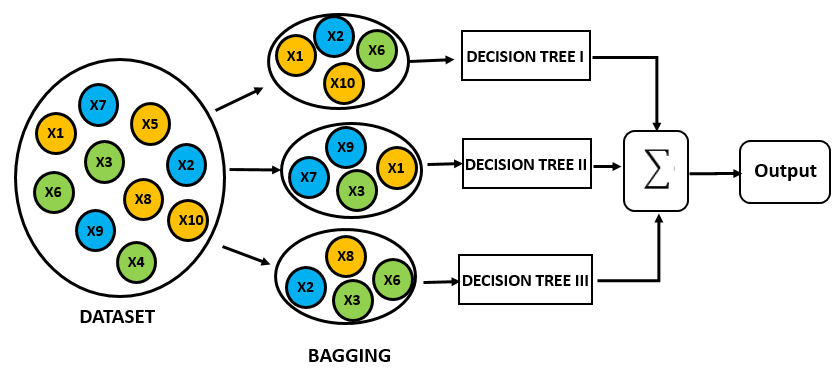
출처: GreyAtom's medium
데이터를 중복추출(with replacement) 방식으로 뽑아내서 여러 tree에 집어넣는 것 뿐 아니라, 각 tree에 사용할 feature 또한 각각 다르게 샘플링한다. 마지막에 각각의 tree가 구분한 결과(classification)를 voting을 통해 집계한다. 몇 개의 tree가 overfitting 되더라도 tree 수가 여러 개 있기 때문에 한 두개 tree의 영향력을 줄일 수 있다는 장점이 있다.
이 프로젝트는 미세먼지 위험 등급을 classification 하는 task이므로 Random Forest를 사용하기 적절하다고 보았다. Sequential 데이터를 다루기 어렵다는 점에서 아쉬움이 있었지만, 데이터셋을 만들 때 timestep T-1의 대기질과 T의 예상되는 날씨를 통해 T의 미세먼지 농도를 구할 수 있도록 조절을 해놓았기 때문에 어느 정도 보완이 되리라 생각한다.
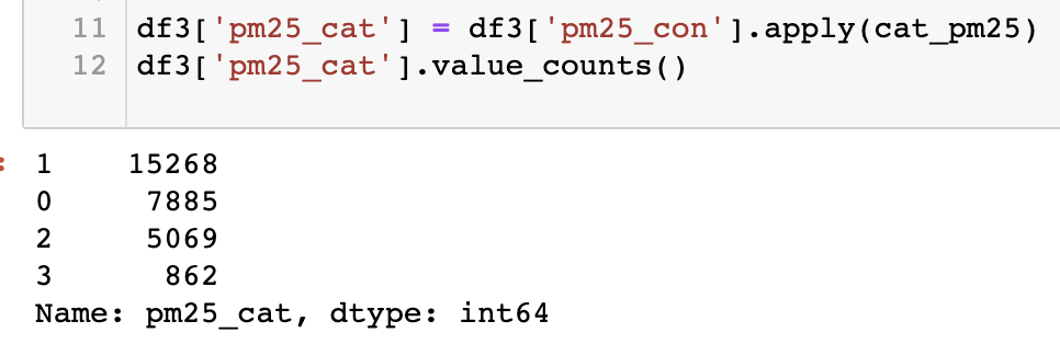
게다가 아래처럼 우리가 원하는 bad, worst 데이터(아래의 2번 3번 데이터)가 적기 때문에 데이터 샘플링 과정에서 쉽게 bad case들의 비중을 높일 수 있게끔 조정할 수 있다는 점도 매력적이었다. 이 부분은 아래 실험하는 부분에서 부연설명하겠다.
Split Test set
앞서 머신러닝을 위해 다듬어둔 데이터에서 test를 위한 test set을 나눈다. 여기서는 test_ratio를 30%로 두었다.
from sklearn.model_selection import train_test_split

X = df.drop('pm25_cat', axis=1)
y = df['pm25_cat']
X_train, X_test, y_train, y_test = train_test_split(X, y, test_size=opt.test_ratio, random_state=SEED)
print('X_train: {:,} \nX_test: {:,}\ny_train: {:,} \ny_test: {:,}'.format(len(X_train), len(X_test), len(y_train),
                                                                  len(y_test)))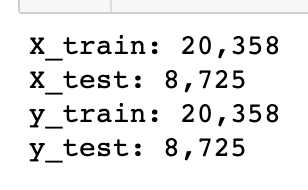
30%로 test set을 구축한 결과 아래처럼 train:test = 20,358:8,725로 분할되었다. feature 데이터와 label을 각각 다른 변수에 할당 후 각각을 다시 train, test로 분할할 때는 torch.utils.data.random_split 보다 sklearn의 train_test_split이 편하다.
Test Metric
시리즈 1번 글에서 이 프로젝트의 목적을 Bad Recall을 높이는 것으로 정의한 바 있다. 따라서 이에 적합한 평가 metric을 만들었다.
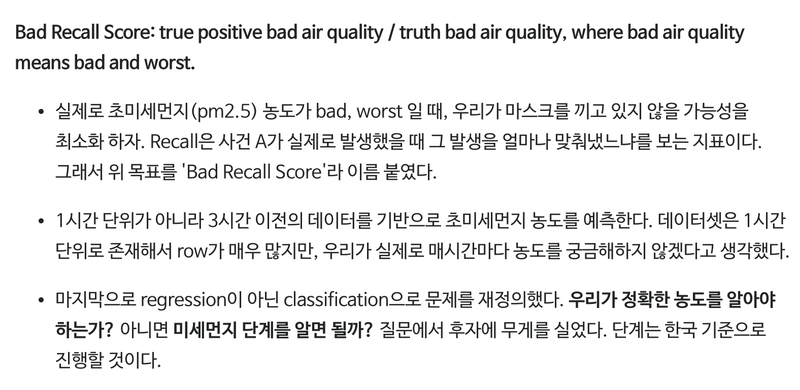
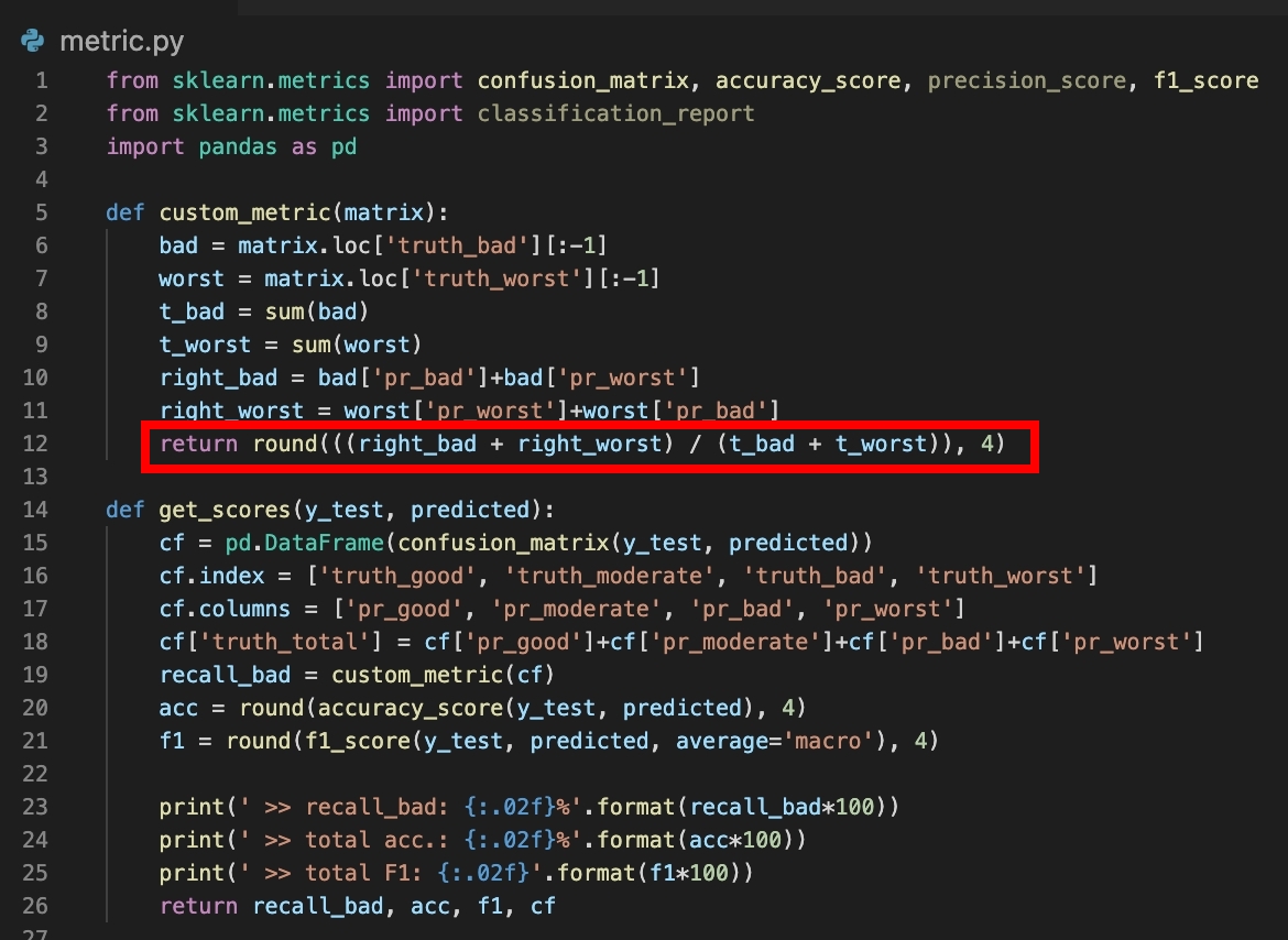
Sklearn의 confusion matrix를 구한 다음, Predict_bad+Predict_worst를 True_bad+True_worst로 나눠주었다. 다시 말해, 실제 bad와 worst 케이스 숫자 중 모델이 bad와 worst로 분류한 숫자의 비율을 구한 것이다. 여기서는 실제 worst인데 bad로 예측한 케이스와 실제 bad인데 worst로 예측한 케이스도 적중한 케이스에 포함된다. 단순 F1 score나 accuracy와는 달리 본 목적에 맞게 customize된 metric인 것이다.
result의 confusion matrix를 봤을 때, {truth_bad and predicted bad(1300) + truth_bad and predicted worst(21) + truth_worst and predicted bad(139) + truth_worst and predicted_worst(85)} / {truth_bad_total(1510) + truth_worst_total(274)} 값이 bad recall score가 된다.
Various weight and max depth
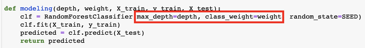
sklearn의 Random Forest는 max_depth와 class_weight을 인자로 받아서 모델링을 수행할 수 있다. max_depth는 말 그대로 tree label의 최대치를 설정하는 인자이다. 최대 깊이를 적절히 조절해줘서 overfit을 방지할 수 있다.
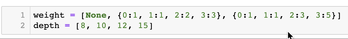
class_weight는 tree에 들어갈 데이터를 sampling with replacement 할 때 각 클래스별로 더 자주 나올 빈도를 주는 것이다. 우리는 bad와 worst를 잡아내는 데 집중해야 하지만 실제 데이터에서는 해당 케이스가 부족하여 이 둘의 weight를 높여보았다. 아래는 실험 목록이다. weight는 세 가지로, depth는 네 가지로 각각 테스트를 해보았으며 이는 총 열두 조합이 된다.
실험을 위한 코드
from sklearn.ensemble import RandomForestClassifier
from sklearn.metrics import confusion_matrix, accuracy_score, precision_score, f1_score
from sklearn.metrics import classification_report

def custom_metric(matrix):
    bad = matrix.loc['truth_bad'][:-1]
    worst = matrix.loc['truth_worst'][:-1]
    t_bad = sum(bad)
    t_worst = sum(worst)
    right_bad = bad['pr_bad']+bad['pr_worst']
    right_worst = worst['pr_worst']+worst['pr_bad']
    return round(((right_bad + right_worst) / (t_bad + t_worst)), 4)

def modeling(depth, weight, X_train, y_train, X_test):
    clf = RandomForestClassifier(max_depth=depth, class_weight=weight, random_state=SEED)
    clf.fit(X_train, y_train)
    predicted = clf.predict(X_test)
    return predicted

def get_scores(y_test, predicted):
    cf = pd.DataFrame(confusion_matrix(y_test, predicted))
    cf.index = ['truth_good', 'truth_moderate', 'truth_bad', 'truth_worst']
    cf.columns = ['pr_good', 'pr_moderate', 'pr_bad', 'pr_worst']
    cf['truth_total'] = cf['pr_good']+cf['pr_moderate']+cf['pr_bad']+cf['pr_worst']
    recall_bad = custom_metric(cf)
    acc = round(accuracy_score(y_test, predicted), 4)
    f1 = round(f1_score(y_test, predicted, average='macro'), 4)

    print(' >> recall_bad: {:.02f}%'.format(recall_bad*100))
    print(' >> total acc.: {:.02f}%'.format(acc*100))
    print(' >> total F1: {:.02f}'.format(f1*100))
    return recall_bad, acc, f1, cf

def run(X_train, y_train, X_test, y_test, depth, weight):
    predicted = modeling(depth, weight, X_train, y_train, X_test)
    print('max_depth: {:} | class_weight: {:}'.format(depth, weight))
    _, _, _, cf = get_scores(y_test, predicted)
    return

weight = [None, {0:1, 1:1, 2:2, 3:3}, {0:1, 1:1, 2:3, 3:5}]
depth = [8, 10, 12, 15]

for i in weight:
    for j in depth:
        run(X_train, y_train, X_test, y_test, j, i)
Result
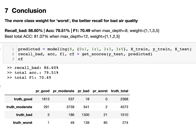
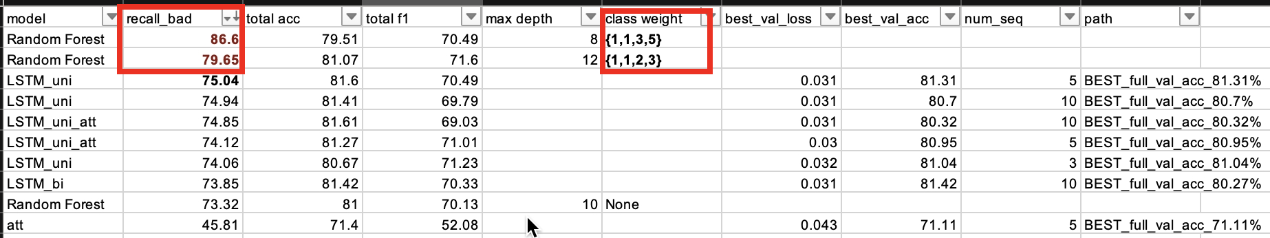
max depth는 8로 class weight는 {1,1,3,5}로 설정했을 때 가장 좋은 bad recall score를 기록했다. bad case에 3의 가중치, worst case에 5의 가중치를 주어 샘플링을 했다는 뜻이다. 데이터를 늘려 학습시킨 만큼 이 둘을 예측하는 데에 좋은 성과를 보였다.
가장 하단의 테이블은 딥러닝 모델을 포함한 모든 실험 결과인데, 학습 과정에서 bad, worst 케이스를 augmentation 했던 것이 간단한 LSTM 모델의 결과보다도 더 좋은 score를 보였던 이유인 듯하다. 다만 종합적인 퍼포먼스(accuracy와 f1 score)는 bad, worst augmentation 정도를 낮추거나 적용하지 않은 모델들에 비해 낮았다. 목적을 가장 잘 이룰 수 있는 모델을 위해 일반적으로 사용되는 퍼포먼스 지표를 trade-off 했다고 할 수 있겠다.
Random Forest 전체 코드는 > github