[MMTA] LSTM Model For Stock Prediction pt.2

Last time, my model was overfitted because I did not handle the noises within the data.

This time, I was inspired by the article: Denoising Stock Price Time Series with Singular Spectrum Analysis for Enhanced Deep Learning Forecasting by Carol Anne Hargreaves and Zixian Fan.

Singular Spectrum Analysis is a technique that adjusts each data points according to its significance in the dataset. It is a very effective method for denoising and feature extracting.

This article also introduced CNN-LSTM hybrid model, where CNN layers is used for feature extraction.

Singular Spectrum Analysis (SSA)

I first created a method for calculating SSA value for a certain range (lookback).

def apply_ssa_trend(series, window = 15, lookback = 60):
    n_total = len(series)
    result = np.zeros(n_total)
    
    result[:lookback] = series[:lookback]
    
    for t in range(lookback, n_total):
        sub_series = series[t - lookback + 1 : t + 1]
        
        N = len(sub_series)
        L = window
        K = N - L + 1
        X = np.column_stack([sub_series[i:i+L] for i in range(K)])
        
        U, Sigma, VT = np.linalg.svd(X, full_matrices=False)
        
        X1 = Sigma[0] * np.outer(U[:, 0], VT[0, :])
        
        n = N - 1
        vals = [X1[i, n-i] for i in range(max(0, n-K+1), min(n+1, L))]
        result[t] = np.mean(vals)
        
    return result

Then I adjusted my get_dataset() method that applies SSA. My previous get_dataset() method applied most of its data preprocessing steps (ex. scaling, column extraction, etc) within two methods, so checking the the dataset for each step was kind of complicated. I separated those steps so that I can analyze the dataset before applying certain steps.

def get_dataset_columns(ticker, period="1y", window=60):
    df = yf.Tickers(ticker).history(period=period)
    vix_data = yf.Tickers("^VIX").history(period=period, progress=False)

    df.columns = df.columns.droplevel(1)
    vix_data.columns = vix_data.columns.droplevel(1)

    df = df.ffill().dropna()

    vix_data = vix_data.reindex(df.index).ffill()

    df = df.drop(['Stock Splits', 'Dividends'], axis=1)

    open_trend = apply_ssa_trend(df['Open'].values, window=int((window/4)))
    vix_trend  = apply_ssa_trend(vix_data['Open'].values, window=int((window/4)))

    min_len = min(len(df), len(open_trend), len(vix_trend))

    df = df.iloc[:min_len]
    df['Open_Trend'] = open_trend[:min_len]
    df['Vix_Trend'] = vix_trend[:min_len]

    df['Trend_Diff'] = df['Open'] - df['Open_Trend']

    df['Target'] = ((df['Close'] - df['Open']) * 100 / df['Open'])
    # df['Target'] = np.log(df['Close'] / df['Open']) * 100
    # df['Target'] = df['Close']

    df = df.drop(df.index[0])
    df = df.drop(['High', 'Low', 'Volume', 'Close'], axis=1)

    feature_cols = ["Open_Trend", "Trend_Diff", "Vix_Trend"]
    target_col = ["Target"]

    return df, feature_cols, target_col

def scale_dataset(df, ticker, feature_cols, target_col, test_size=0.2, scale_target=False):
    train_size = int(len(df) * (1 - test_size))
    df_train = df.iloc[:train_size]

    if ticker not in feature_scalers:
        f_scaler = StandardScaler()
        f_scaler.fit(df_train[feature_cols])
        feature_scalers[ticker] = f_scaler

        if scale_target:
            t_scaler = StandardScaler()
            t_scaler.fit(df_train[target_col]) 
            target_scalers[ticker] = t_scaler

    df[feature_cols] = feature_scalers[ticker].transform(df[feature_cols])
    if scale_target:
        df[target_col] = target_scalers[ticker].transform(df[target_col])

    data_x = df[feature_cols].values
    data_y = df[target_col].values

    return data_x, data_y    

def get_full_dataset(tickers, period="1y", window_size=60, test_size=0.2):
    X_total, y_total = [], []
    
    for ticker in tickers:
        df, feature_cols, target_col = get_dataset_columns(ticker, period=period, window=window_size)
        data_x, data_y = scale_dataset(df, ticker, feature_cols, target_col, test_size, scale_target=False)
        
        for i in range(len(df) - window_size):
            X_total.append(data_x[i : i + window_size])
            y_total.append(data_y[i + window_size])

    X_data = np.array(X_total)
    y_data = np.array(y_total)

    nan_mask = np.isnan(X_data).any(axis=(1, 2))
    X_data = X_data[~nan_mask]
    y_data = y_data[~nan_mask] 

    print(f"NaN Deleted: {np.sum(nan_mask)}")
    
    test_first_index = int(len(X_data) * (1 - test_size))
    X_train, X_test = X_data[:test_first_index], X_data[test_first_index:]
    y_train, y_test = y_data[:test_first_index], y_data[test_first_index:]

    print("""
    X_train Shape : {}
    X_test Shape : {}
    y_train Shape : {}
    y_test Shape : {}
    """.format(X_train.shape, X_test.shape, y_train.shape, y_test.shape))
    
    return X_train, X_test, y_train, y_test

The resulting dataset would now have a “Open” column and “Open Trend” that would look like this:

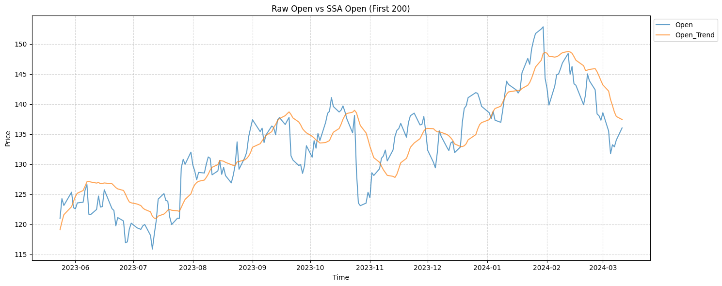
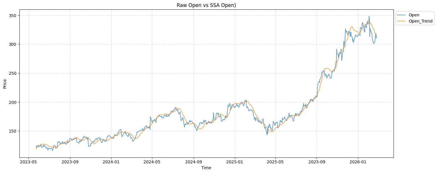
It looks like it is lagging because each values are calculated based on the average movement of the past 60 days. To address this problem, I added another column "Trend_Diff" that represents the noise within the trend.

CNN-LSTM Hybrid Model

This is the CNN-LSTM model I chose.

def get_CNN_LSTM_hybrid(window_size=60, feature_num=7):
    dropout_rate = 0.2
    
    input_layer = Input(shape=(window_size, feature_num), name="Input")
    
    x = Conv1D(filters=64, kernel_size=3, strides=1, padding='same', activation='relu', name="Conv1D_1")(input_layer)
    x = LayerNormalization(name="LayerNormalization_1")(x)
    x = Conv1D(filters=64, kernel_size=3, strides=1, padding='same', activation='relu', name="Conv1D_2")(x)
    x = LayerNormalization(name="LayerNormalization_2")(x)
    
    x = MaxPooling1D(pool_size=2, name="Max_Pooling")(x)
    
    x = LSTM(64, return_sequences=True, name="LSTM_1")(x)
    x = Dropout(dropout_rate, name="Dropout_1")(x)
    x = BatchNormalization(name="BatchNormalization_1")(x)
    
    x = LSTM(32, return_sequences=False, name="LSTM_2")(x)
    x = Dropout(dropout_rate, name="Dropout_2")(x)
    x = BatchNormalization(name="BatchNormalization_2")(x)
    
    x = Dense(16, activation="relu", name="FullyConnected_1")(x)
    output_layer = Dense(1, activation="linear", name="Output")(x)

    model = Model(inputs=input_layer, outputs=output_layer, name='SSA_CNN_LSTM_Hybrid')

    optimizer = tf.keras.optimizers.Adam(learning_rate=0.001)
    model.compile(optimizer=optimizer, 
                  loss='mse', 
                  metrics=['mae', tf.keras.metrics.RootMeanSquaredError()])
    return model

CNN_LSTM_model = get_CNN_LSTM_hybrid(window_size, feature_num)
CNN_LSTM_model.summary()

This is the previous LSTM model I will be comparing to:

def get_LSTM_model(window_size=60, feature_num=7):
    dropout_rate = 0.2
    input_layer = Input(shape = (window_size, feature_num), name="Input")
    batch_norm_layer = BatchNormalization(name="BatchNormalization_1")(input_layer)
    LSTM_layer = LSTM(64, return_sequences=True, name = "LSTM_1")(batch_norm_layer)
    hidden_layer = Dropout(dropout_rate, name = f"Dropout_1_{dropout_rate}")(LSTM_layer)
    hidden_layer = BatchNormalization(name="BatchNormalization_2")(hidden_layer)
    hidden_layer = LSTM(32, name = "LSTM_2")(hidden_layer)
    hidden_layer = Dropout(dropout_rate, name = f"Dropout_2_{dropout_rate}")(hidden_layer)
    hidden_layer = Dense(16, activation = "relu", name="Dense")(hidden_layer)
    output_layer = Dense(1, activation = "linear", name="Output")(hidden_layer)

    model = Model(inputs = input_layer, outputs = output_layer, name='LSTM_BatchNorm_Dropout0.2_3y_window30')

    optimizer = tf.keras.optimizers.Adam(learning_rate=0.0001)
    # loss_fn = tf.keras.losses.Huber()
    model.compile(optimizer = optimizer, loss = 'mse', metrics=['mae', tf.keras.metrics.RootMeanSquaredError()])
    return model

LSTM_model = get_LSTM_model(window_size, feature_num)
LSTM_model.summary()

---

Results:

I trained the model with the same companies as last time.

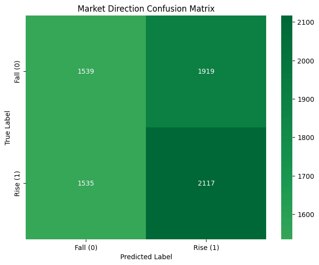
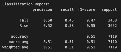
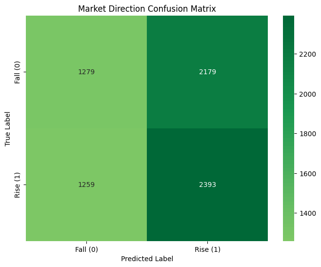
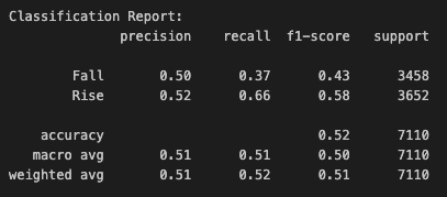
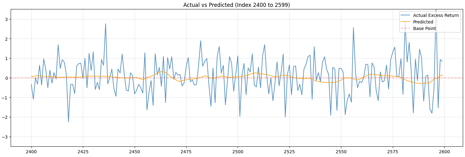
These are the results for CNN-LSTM model:

These only represent the classification of whether the price will rise or not.

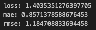
These are the metrics regarding the value:

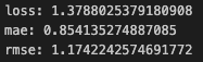
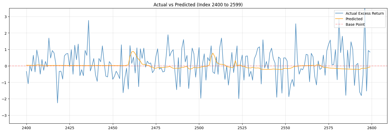
Although the model is terrible at predicting, I see this as a huge improvement.

The previous LSTM model only predicted the value to be rising and the orange line was just a straight line. It is now predicting more diversely.

These are the results for previous LSTM model:

The LSTM model’s predictions have also shown improvements, but are still kind of overfitted. This still means that SSA is actually helping address overfitting problem.

---

The results show that applying SSA method and implementing CNN-LSTM model helped addressing overfitting problem.

Next time, I will be trying to improve the accuracy. I think I will be trying to add diffusion model in-between, but more research is required (if I find something that seems to be more effective, I might implement that).

---

Reference:
Hargreaves, C. A., & Fan, Z. (2026). Denoising Stock Price Time Series with Singular Spectrum Analysis for Enhanced Deep Learning Forecasting. Analytics, 5(1), 9. https://doi.org/10.3390/analytics5010009