[MMTA] LSTM Model For Stock Prediction

My current BERT model is generating the same output for any input, and I wasn’t able to find the reason behind it. So I started working on my LSTM model for a bit of mental refresh.

Output of this model and the BERT model will be inputted into an LLM, which will decide to buy/hold/sell the stock.

---

I first started by collecting data. I used yfinance library collect stock data.

Then added / removed features for the dataset. I am still deciding which features to be added and which metric should be set as the target.

def get_dataset(ticker, period="1y"):
    df = yf.Tickers(ticker).history(period = period)
    df.columns = df.columns.droplevel(1)
    df = df.ffill().dropna()

    df = df.drop(['Stock Splits', 'Dividends'], axis=1)
    df['Yesterday_High'] = df['High'].shift(1)
    df['Yesterday_Low'] = df['Low'].shift(1)
    df['Yesterday_Volume'] = df['Volume'].shift(1)
    df['Yesterday_Close'] = df['Close'].shift(1)
    # df['Return'] = ((df['Close'] - df['Yesterday_Close'])  * 100 / df['Yesterday_Close'])
    df['Return'] = np.log(df['Close'] / df['Yesterday_Close']) * 100
    df = df.drop(df.index[0])
    
    df = df.drop(['High', 'Low', 'Volume', 'Close'], axis=1)

    return df

Then I scaled the dataset using StandardScaler , which scales the value so that the mean of the dataset is 0 and standard deviation is 1. I tried to make sure that the information about the testing datasets wasn’t given to the scaler so that the scaling does not include any information about the future.

Then I converted the time series data into a supervised learning format using sliding window approach.

def get_full_dataset(tickers, period="1mo", window_size=60, test_size=0.2):
    X_total, y_total = [], []
    
    for ticker in tickers:
        df = get_dataset(ticker, period)
        feature_cols = ['Open', 'Yesterday_High', 'Yesterday_Low', 'Yesterday_Volume', 'Yesterday_Close']
        target_col = ['Return']

        train_size = int(len(df) * (1 - test_size))
        df_train = df.iloc[:train_size]

        if ticker not in feature_scalers:
            f_scaler = StandardScaler()
            f_scaler.fit(df_train[feature_cols])
            feature_scalers[ticker] = f_scaler
            
            # t_scaler = StandardScaler()
            # t_scaler.fit(df_train[target_col]) 
            target_scalers[ticker] = t_scaler

        df[feature_cols] = feature_scalers[ticker].transform(df[feature_cols])
        df[target_col] = target_scalers[ticker].transform(df[target_col])

        data_x = df[feature_cols].values
        data_y = df[target_col].values
        
        for i in range(len(df) - window_size):
            X_total.append(data_x[i : i + window_size])
            y_total.append(data_y[i + window_size])

    X_data = np.array(X_total)
    y_data = np.array(y_total)

    nan_mask = np.isnan(X_data).any(axis=(1, 2))
    X_data = X_data[~nan_mask]
    y_data = y_data[~nan_mask] 

    print(f"NaN Deleted: {np.sum(nan_mask)}")
    
    test_first_index = int(len(X_data) * (1 - test_size))
    X_train, X_test = X_data[:test_first_index], X_data[test_first_index:]
    y_train, y_test = y_data[:test_first_index], y_data[test_first_index:]

    print("""
    X_train Shape : {}
    X_test Shape : {}
    y_train Shape : {}
    y_test Shape : {}
    """.format(X_train.shape, X_test.shape, y_train.shape, y_test.shape))
    
    return X_train, X_test, y_train, y_test

I collected data from 50 different companies.

tickers_50 = [
    "AAPL", "MSFT", "GOOGL", "AMZN", "META", "TSLA", "NFLX", "ADBE", "CRM", "ORCL",
    "NVDA", "TSM", "AVGO", "ASML", "AMD", "INTC", "QCOM", "TXN", "MU", "AMAT",
    "JPM", "BAC", "V", "MA", "GS", "MS", "AXP", "PYPL", "WFC", "BLK",
    "JNJ", "LLY", "UNH", "PFE", "ABBV", "MRK", "TMO", "DHR", "AMGN", "ISRG",
    "PG", "KO", "PEP", "WMT", "COST", "NKE", "MCD", "HD", "DIS", "SBUX"
]

window_size = 60

X_train, X_test, y_train, y_test = get_full_dataset(
    tickers_20,
    period = "6y",
    window_size = window_size, 
    test_size = 0.2
)

def get_LSTM_model(window_size=60, feature_num=7):
    dropout_rate = 0.2
    input_layer = Input(shape = (window_size, feature_num), name="Input")
    batch_norm_layer = BatchNormalization(name="BatchNormalization_1")(input_layer)
    LSTM_layer = LSTM(64, return_sequences=True, name = "LSTM_1")(batch_norm_layer)
    hidden_layer = Dropout(dropout_rate, name = f"Dropout_1_{dropout_rate}")(LSTM_layer)
    hidden_layer = BatchNormalization(name="BatchNormalization_2")(hidden_layer)
    hidden_layer = LSTM(64, return_sequences=True, name = "LSTM_2")(hidden_layer)
    hidden_layer = Dropout(dropout_rate, name = f"Dropout_2_{dropout_rate}")(hidden_layer)
    hidden_layer = BatchNormalization(name="BatchNormalization_3")(hidden_layer)
    hidden_layer = LSTM(32, return_sequences=True, name = "LSTM_3")(hidden_layer)
    hidden_layer = Dropout(dropout_rate, name = f"Dropout_3_{dropout_rate}")(hidden_layer)
    hidden_layer = LSTM(32, name = "LSTM_4")(hidden_layer)
    hidden_layer = Dropout(dropout_rate, name = f"Dropout_4_{dropout_rate}")(hidden_layer)
    hidden_layer = Dense(16, activation = "relu", name="Dense")(hidden_layer)
    output_layer = Dense(1, activation = "linear", name="Output")(hidden_layer)

    model = Model(inputs = input_layer, outputs = output_layer, name='LSTM_BatchNorm_Dropout0.2_3y_window30')

    optimizer = tf.keras.optimizers.Adam(learning_rate=0.0001)
    # loss_fn = tf.keras.losses.Huber()
    model.compile(optimizer = optimizer, loss = 'mse', metrics=['mae', tf.keras.metrics.RootMeanSquaredError()])
    return model

LSTM_model.fit(
    X_train, 
    y_train, 
    epochs = 50, 
    batch_size = 32,
    validation_data = (X_test, y_test),
    callbacks = [earlyStopping_callback]
)

---

These are the results of the model :

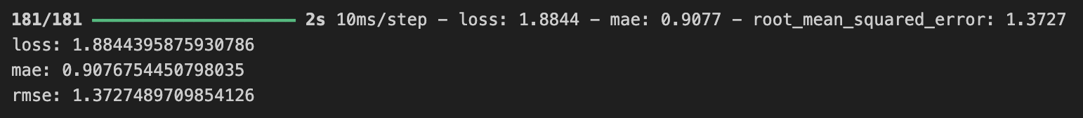
Considering that the model is predicting the logarithmic return where the standard deviation is around 2.3, mae score of 0.9 implies that the model is not performing well at all.

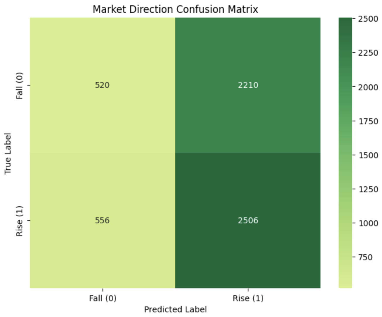
This confusion matrix shows that the model is overfitted to predict that the stock will increase.

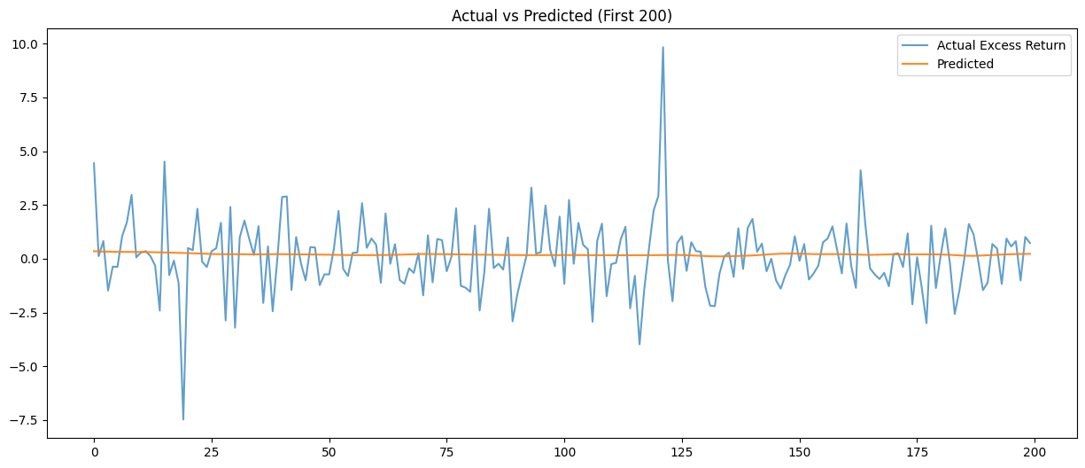
The magnitude of the model’s predictions is gathered around the 0-line, once again implying that the model is overfitted.

However, the model was expected to be overfitted as noises in the stock data weren’t handled. For the next couple of days, I plan to study several denoising techniques and apply it to my model.