weights 최적값 찾기 - Gradient Descent

👉정해야 하는 것
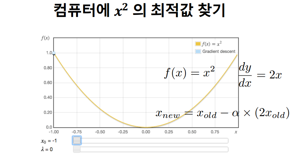
1) (한 번에 얼마만큼 갈것인지)Learning rate에 대한 선정 : α
2) 얼마나 많이 loop를 돌 것인가? : 너무 많지 않고 적지 않게
📌 wolframealpha.com 미분값과 그래프 쉽게 만드는 사이트
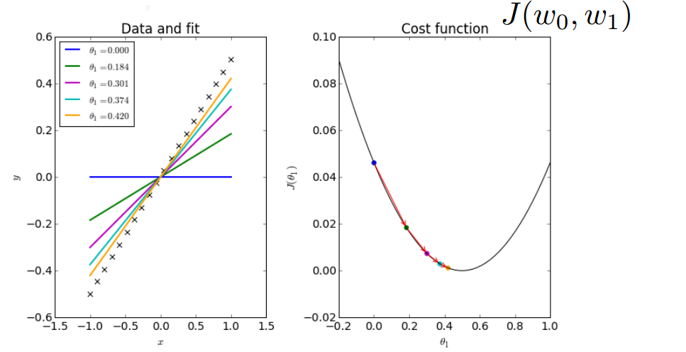실제 그래프에 예측치가 가까워지는 것을 알 수 있다.

⇒ parameter(w0,w1로 학습을 통해 알아내는 것)를 업데이트 시켜주면서 오차를 줄인다.

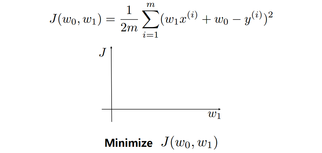
Linear regression with GD

임의의 θ1, θ2값으로 초기화해준다.
cost function J가 최소화 될 때가지 학습시킨다.
더이상 cost function이 줄어들지 않거나 학습 횟수를 초과할 때 종료시킨다.
Learning rate Iteration 횟수 등 Parameter 지정
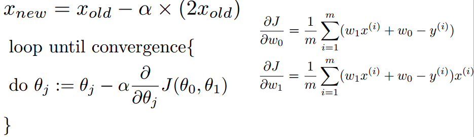w0,w1의 값을 동시에 업데이트 시켜줘야 한다. 즉 새로운 값끼리 연산을 따로 한다.

import matplotlib.pyplot as plt
%matplotlib inline
import pandas as pd
import numpy as np

df = pd.read_csv("data/slr06.csv")
df.head()

raw_X = df["X"].values.reshape(-1, 1)
y = df["Y"].values

plt.figure(figsize=(10,5))
plt.plot(raw_X,y, 'o', alpha=0.5)

raw_X[:5], y[:5]
np.ones((len(raw_X),1))[:3]
X = np.concatenate( (np.ones((len(raw_X),1)), raw_X ), axis=1)
X[:5]
w = np.random.normal((2,1)) 
# w = np.array([5,3])
w
plt.figure(figsize=(10,5))
y_predict = np.dot(X, w)
plt.plot(raw_X,y,"o", alpha=0.5)
plt.plot(raw_X,y_predict)

def hypothesis_function(X, theta):
    return X.dot(theta)
h = hypothesis_function(X,w)
def cost_function(h, y):
    return (1/(2*len(y))) * np.sum((h-y)**2)
h = hypothesis_function(X,w)
cost_function(h, y)

def gradient_descent(X, y, w, alpha, iterations): #y:bias, x0:1, x1:1~100, iterations:몇번 돌건지
    theta = w 
    m = len(y) #데이터의 총 개수
    
    theta_list = [theta.tolist()]
    cost = cost_function(hypothesis_function(X, theta), y)

    for i in range(iterations):
        t0 = theta[0] - (alpha / m) * np.sum(np.dot(X, theta) - y)
        t1 = theta[1] - (alpha / m) * np.sum((np.dot(X, theta) - y) * X[:,1])
        theta = np.array([t0, t1])
        
        if i % 10== 0:
            theta_list.append(theta.tolist())
            cost = cost_function(hypothesis_function(X, theta), y)
            cost_list.append(cost)


    return theta, theta_list, cost_list

iterations = 10000
alpha = 0.001

theta, theta_list, cost_list = gradient_descent(X, y, w, alpha, iterations)
cost = cost_function(hypothesis_function(X, theta), y)

print("theta:", theta)
print('cost:', cost_function(hypothesis_function(X, theta), y))
theta_list[:10]
theta_list = np.array(theta_list)
cost_list[:5]

plt.figure(figsize=(10,5))

y_predict_step= np.dot(X, theta_list.transpose())

y_predict_step
plt.plot(raw_X,y,"o", alpha=0.5)
for i in range (0,len(cost_list),100):
    plt.plot(raw_X,y_predict_step[:,i], label='Line %d'%i)

plt.legend(bbox_to_anchor=(1.05, 1), loc=2, borderaxespad=0.)
plt.show()

✔ feature가 여러개일 경우 Multivariate Linear Regression 사용