Tensorflow와 Keras를 이용한 딥러닝 구현(2)

딥러닝 구현과 MNIST데이터를 활용한 모델 학습

from tensorflow.keras import Sequential
from tensorflow.keras.layers import Dense

# 손글씨 숫자 이미지로 구성된 MNIST 데이터셋
from tensorflow.keras.datasets import mnist
# 정답을 원핫 인코딩하기 위한 함수
from tensorflow.keras.utils import to_categorical

import matplotlib.pyplot as plt

# 훈련 데이터 60000개와 테스트 데이터 10000개를 불러옵니다.
(x_data, y_data), (x_test, y_test) = mnist.load_data()

# 28×28 이미지를 길이가 784인 1차원 벡터로 변환
# 픽셀값을 255로 나누어 0~1 범위로 정규화
x_data = x_data.reshape(-1, 784).astype("float32") / 255.0
x_test = x_test.reshape(-1, 784).astype("float32") / 255.0

# 전체 훈련 데이터 중 앞의 50000개를 실제 훈련에 사용
x_train = x_data[:-10000]

# 마지막 10000개를 검증 데이터로 사용합니다.
x_val = x_data[-10000:]

# 입력 데이터와 같은 기준으로 정답 데이터를 분리합니다.
y_train = y_data[:-10000]
y_val = y_data[-10000:]

# 숫자 형태의 정답을 길이가 10인 원-핫 벡터로 변환합니다.
y_train_encoded = to_categorical(y_train, num_classes=10)
y_val_encoded = to_categorical(y_val, num_classes=10)
y_test_encoded = to_categorical(y_test, num_classes=10)


model = Sequential()

model.add(Dense(100, activation="sigmoid"))
# 숫자 0~9를 분류하기 위해 출력 뉴런을 10개로 설정합니다.
# 소프트맥스 함수는 각 클래스에 속할 확률을 출력합니다.
model.add(Dense(10, activation="softmax"))


model.compile(
    optimizer="sgd",
    loss="categorical_crossentropy",
    metrics=["accuracy"]
)

history = model.fit(
    x_train,
    y_train_encoded,
    epochs=40,
    validation_data=(x_val, y_val_encoded)
)

plt.plot(history.history["loss"])
plt.plot(history.history["val_loss"])
plt.ylabel("loss")
plt.xlabel("epoch")
plt.legend(["train_loss", "val_loss"])
plt.show()

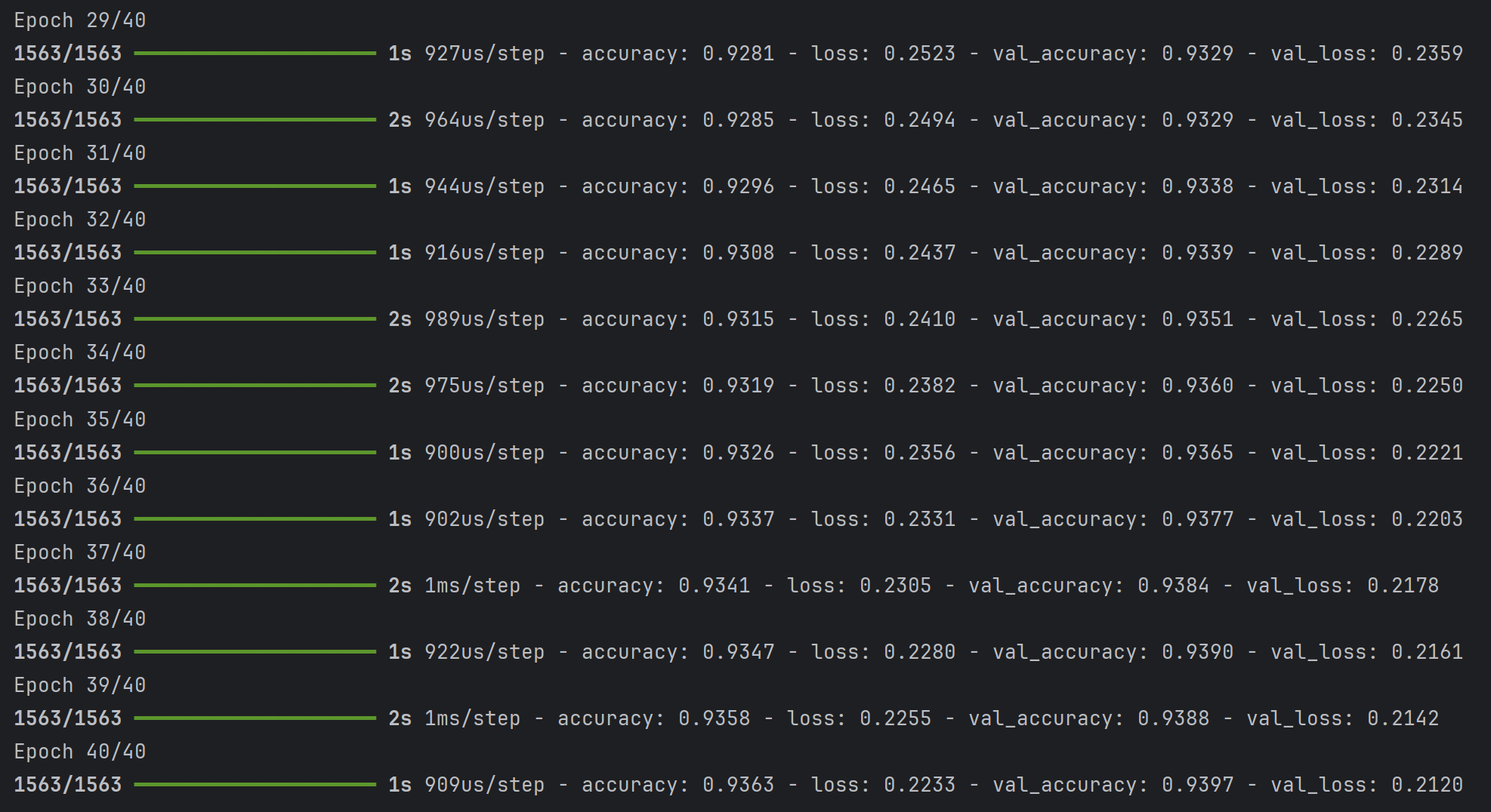
실행해보면

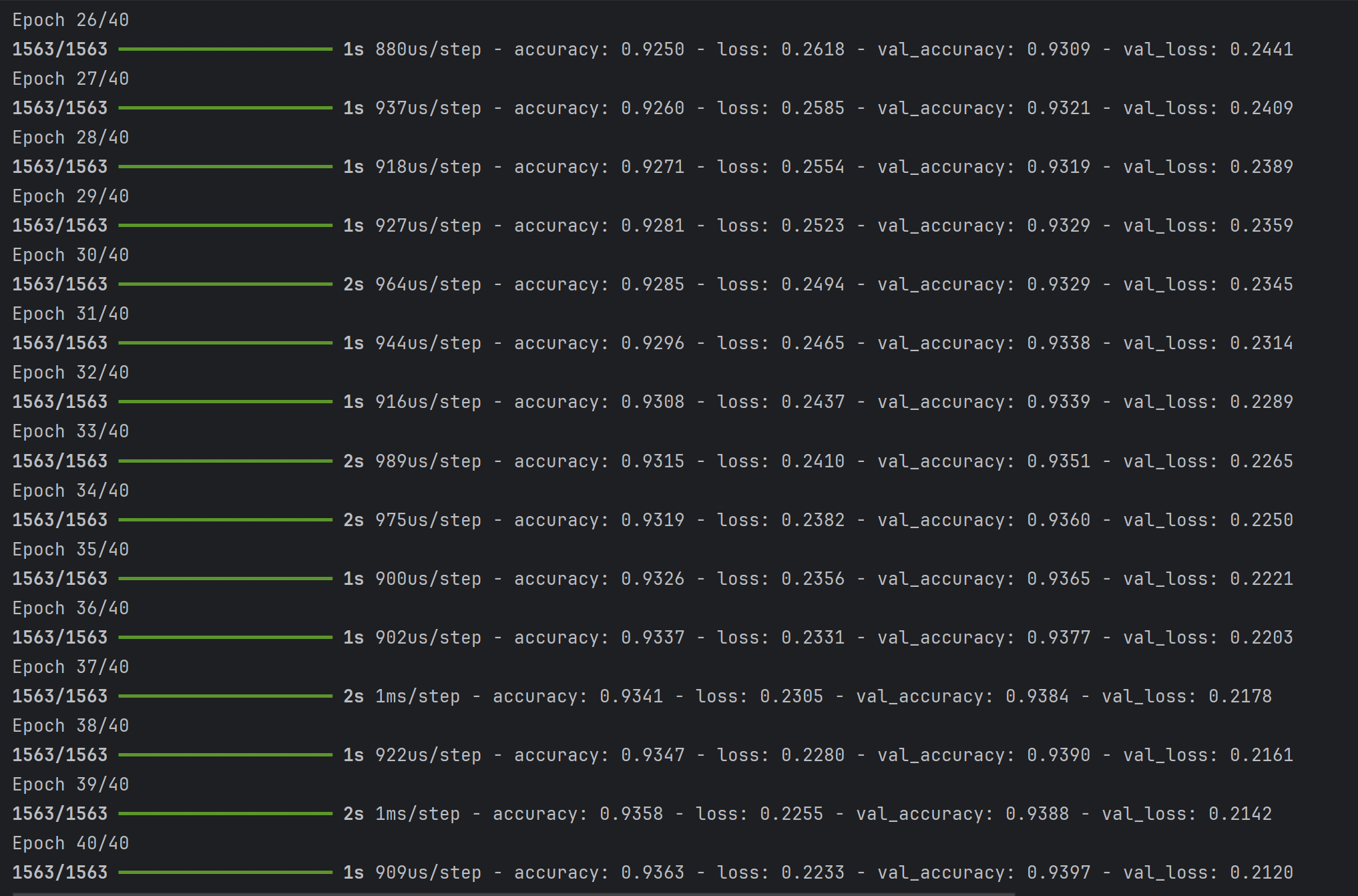
다음과 같이 에포크별 accuracy, loss값을 확인할 수 있고

마지막에 pyplot으로 그려진 그래프 확인할 수 있습니다.

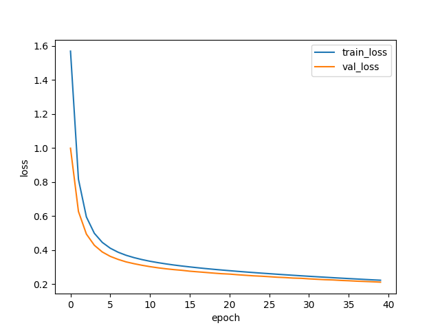
accuracy를 나타내는 그래프를 보고 싶다면 밑부분을

plt.plot(history.history["accuracy"])
plt.plot(history.history["val_accuracy"])
plt.ylabel("accuracy")
plt.xlabel("epoch")
plt.legend(["train_accuracy", "val_accuracy"])
plt.show()

다음과 같이 바꾸면

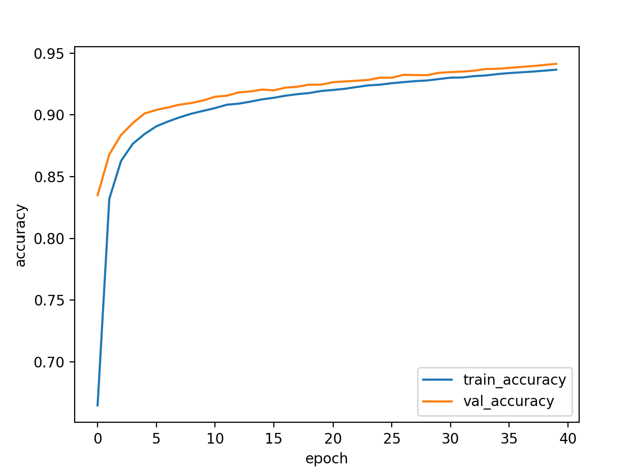
accuracy 그래프까지 확인할 수 있습니다.