Many to Many란?

Many to Many는 자연어 처리에서 개체명 인식, 형태소 분석과 같은 스퀀스 태깅 등에 활용할 수 있다.

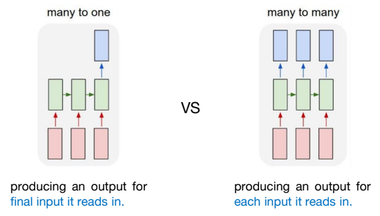
Many to One은 각 토큰을 읽다가 마지막 토큰을 읽었을 때 출력을 내는 구조였다.

그러나 Many to Many는 시퀀스 각각의 토큰에 대해서 출력을 내는 방식이다.

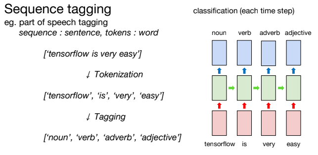
위 형태소 분석 예제에서, 먼저 ['tensorflow is very easy']라는 문장이 주어졌을 때 이를 Tokenization 한다.

['tensorflow is very easy']
=> Tokenization
= ['tensorflow', 'is', 'very', 'easy']

토큰으로 이루어진 시퀀스를 읽고 해당 토큰이 어떤 품사인지를 파악하는 방식으로 Many to Many를 활용할 수 있다.

---

구현 예제

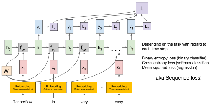
마찬가지로, 각 토큰을 읽을 수 있도록 Embedding layer를 거치게 한다.

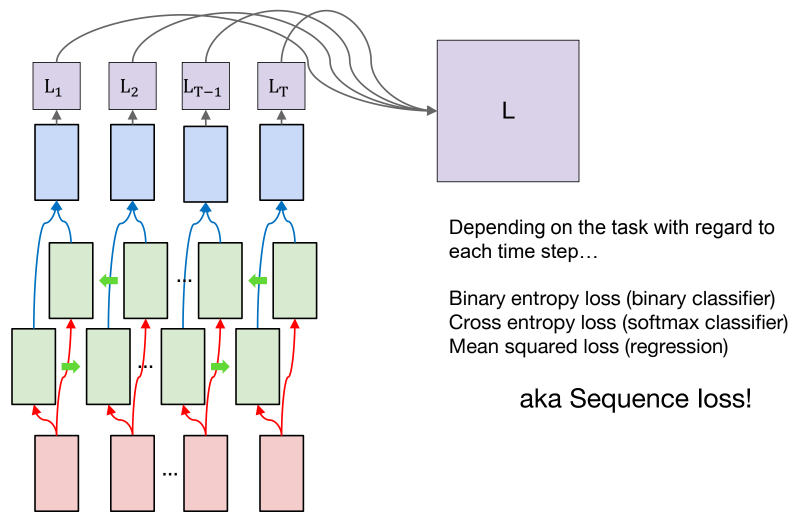
RNN은 순서대로 토큰을 읽고 토큰에 대한 출력을 내고, 이를 정답과 비교하여 토큰마다 loss를 계산한다.

출력된 토큰의 loss 평균을 내는 걸 시퀀스 로스라고 하는데, 이 시퀀스 로스를 통해 backpropagation 하여 학습을 진행하게 된다.

이때 loss 계산이 복잡해지게 된다. 특히 시퀀스 길이를 맞추기 위한 pad 토큰을 고려해야 한다.

=> 따라서 데이터의 시퀀스 토큰 중, pad 토큰에 대해서 loss를 계산하지 않는 masking을 사용하게 된다.

---

구현 코드

1. 데이터셋 준비

import numpy as np
import tensorflow as tf
from tensorflow import keras
from tensorflow.keras import layers
from tensorflow.keras.models import Sequential
from tensorflow.keras.preprocessing.sequence import pad_sequences
from pprint import pprint
import matplotlib.pyplot as plt

# example data
sentences = [
    ['I', 'feel', 'hungry'],
    ['tensorflow', 'is', 'very', 'difficult'],
    ['tensorflow', 'is', 'a', 'framework', 'for', 'deep', 'learning'],
    ['tensorflow', 'is', 'very', 'fast', 'changing'],
]
pos = [
    ['pronoun', 'verb', 'adjective'],
    ['noun', 'verb', 'adverb', 'adjective'],
    ['noun', 'verb', 'determiner', 'noun', 'preposition', 'adjective', 'noun'],
    ['noun', 'verb', 'adverb', 'adjective', 'verb'],
]

# creating a token dictionary for word
word_list = sum(sentences, [])
word_list = sorted(set(word_list))
word_list = ['<pad>'] + word_list
word2idx = {word: idx for idx, word in enumerate(word_list)}
idx2word = {idx: word for idx, word in enumerate(word_list)}

print(word2idx)
print(idx2word)
print(len(idx2word))

# creating a token dictionary for part of speech
pos_list = sum(pos, [])
pos_list = sorted(set(pos_list))
pos_list = ['<pad>'] + pos_list
pos2idx = {pos: idx for idx, pos in enumerate(pos_list)}
idx2pos = {idx: pos for idx, pos in enumerate(pos_list)}

print(pos2idx)
print(idx2pos)
print(len(pos2idx))

# converting sequence of tokens to sequence of indices
max_sequence = 10
x_data = list(map(lambda sentence: [word2idx.get(token) for token in sentence], sentences))
y_data = list(map(lambda sentence: [pos2idx.get(token) for token in sentence], pos))

# padding the sequence of indices
x_data = pad_sequences(sequences=x_data, maxlen=max_sequence, padding='post')
x_data_mask = ((x_data != 0) * 1).astype(np.float32)  # 패딩한 부분에 대한 마스킹 정보를 담음
x_data_len = list(map(lambda sentence: len(sentence), sentences))  # 토크나이제이션 되었을 때 문장의 유효한 길이

y_data = pad_sequences(sequences=y_data, maxlen=max_sequence, padding='post')

# checking data
print(x_data, x_data_len)
print(x_data_mask)
print(y_data)

---

2. 모델 생성

# creating rnn for "many to many" sequence tagging
num_classes = len(pos2idx)
hidden_dim = 10

input_dim = len(word2idx)
output_dim = len(word2idx)
one_hot = np.eye(len(word2idx))

model = Sequential()
model.add(
    layers.Embedding(
        input_dim=input_dim,
        output_dim=output_dim,
        mask_zero=True,
        trainable=False,
        input_length=max_sequence,
        embeddings_initializer=keras.initializers.Constant(one_hot),
    )
)

# return_sequences=True : rnn이 모든 토큰에 대해 출력을 내야하기 때문이다.
model.add(layers.SimpleRNN(units=hidden_dim, return_sequences=True))

# TimeDistributed + Dense를 사용해 매 토큰마다 품사가 무엇인지 분류한다.
model.add(layers.TimeDistributed(layers.Dense(units=num_classes)))

model.summary()

=> 결과

Layer (type)	Output Shape	Param #
embedding (Embedding)	(None, 10, 15)	225
simple_rnn (SimpleRNN)	(None, 10, 10)	260
time_distributed (TimeDistributed)	(None, 10, 8)	88

항목	값
Total params	573
Trainable params	348
Non-trainable params	225

---

3. 모델 학습

# creating loss function
# 매 토큰마다 loss를 계산해야 하고, 특히 pad 토큰에 대해서는 계산하면 안되기 때문에
# 시퀀스의 유효한 길이(x_len)와 max_sequence를 받아 masking을 생성하고 이를 미니배치 loss에 반영한다.

# reduction을 NONE으로 두면 (batch, time) 형태로 토큰별 loss를 얻을 수 있다.
loss_obj = tf.keras.losses.SparseCategoricalCrossentropy(
    from_logits=True,
    reduction=tf.keras.losses.Reduction.NONE,
)

def loss_fn(model, x, y, x_len, max_sequence):  # pad를 제외한 sequence loss 계산 목적
    logits = model(x, training=True)  # (batch, time, num_classes)

    # 토큰별 loss: (batch, time)
    per_token_loss = loss_obj(y_true=y, y_pred=logits)

    # pad 제외용 masking: (batch, time)
    masking = tf.sequence_mask(x_len, maxlen=max_sequence, dtype=tf.float32)

    # pad 위치 loss=0
    per_token_loss = per_token_loss * masking

    # 샘플별 평균 loss: time축 합 -> 유효길이로 나눔
    valid_time_step = tf.cast(x_len, dtype=tf.float32)
    loss_per_sample = tf.reduce_sum(per_token_loss, axis=-1) / valid_time_step

    # 미니배치 평균
    sequence_loss = tf.reduce_mean(loss_per_sample)
    return sequence_loss

# creating an optimizer
lr = 0.1
epochs = 30
batch_size = 2
opt = tf.keras.optimizers.Adam(learning_rate=lr)

# generating data pipeline
tr_dataset = tf.data.Dataset.from_tensor_slices((x_data, y_data, x_data_len))
tr_dataset = tr_dataset.shuffle(buffer_size=4)
tr_dataset = tr_dataset.batch(batch_size=batch_size)

print(tr_dataset)
# <BatchDataset shapes: ((?, 10), (?, 10), (?,)), types: (tf.int32, tf.int32, tf.int32)>

# training
tr_loss_hist = []

for epoch in range(epochs):
    avg_tr_loss = 0.0
    tr_step = 0

    for x_mb, y_mb, x_mb_len in tr_dataset:
        with tf.GradientTape() as tape:
            # 이전 예제와는 다르게, loss func가 유효길이 x_len과 최대 시퀀스 max_sequence를 받는다.
            tr_loss = loss_fn(model, x=x_mb, y=y_mb, x_len=x_mb_len, max_sequence=max_sequence)

        grads = tape.gradient(target=tr_loss, sources=model.trainable_variables)
        opt.apply_gradients(grads_and_vars=zip(grads, model.trainable_variables))

        avg_tr_loss += float(tr_loss)
        tr_step += 1

    avg_tr_loss /= tr_step
    tr_loss_hist.append(avg_tr_loss)

    if (epoch + 1) % 5 == 0:
        print('epoch : {:3}, tr_loss : {:.3f}'.format(epoch + 1, avg_tr_loss))

=> 출력 결과 (예시)
epoch : 5, tr_loss : 0.249
epoch : 10, tr_loss : 0.040
epoch : 15, tr_loss : 0.006
epoch : 20, tr_loss : 0.002
epoch : 25, tr_loss : 0.001
epoch : 30, tr_loss : 0.001

---

4. 정확도 확인

yhat = model.predict(x_data, verbose=0)
yhat = np.argmax(yhat, axis=-1) * x_data_mask

pprint(list(map(lambda row: [idx2pos.get(elm) for elm in row], yhat.astype(np.int32).tolist())), width=120)
pprint(pos)

plt.plot(tr_loss_hist)
plt.show()

=> 결과 (예시)

# 모델의 결과
[['pronoun', 'verb', 'adjective', '<pad>', '<pad>', '<pad>', '<pad>', '<pad>', '<pad>', '<pad>'],
 ['noun', 'verb', 'adverb', 'adjective', '<pad>', '<pad>', '<pad>', '<pad>', '<pad>', '<pad>'],
 ['noun', 'verb', 'determiner', 'noun', 'preposition', 'adjective', 'noun', '<pad>', '<pad>', '<pad>'],
 ['noun', 'verb', 'adverb', 'adjective', 'verb', '<pad>', '<pad>', '<pad>', '<pad>', '<pad>']]

# 모델의 정답
[['pronoun', 'verb', 'adjective'],
 ['noun', 'verb', 'adverb', 'adjective'],
 ['noun', 'verb', 'determiner', 'noun', 'preposition', 'adjective', 'noun'],
 ['noun', 'verb', 'adverb', 'adjective', 'verb']]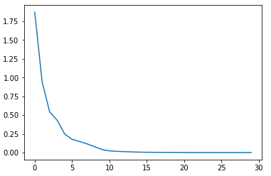

---

Lec-00. bidirectional이란?

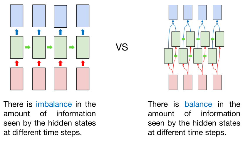
• 기존에는 RNN을 모두 단방향으로만 활용하였고, 특히 RNN을 Many to Many로 활용할 때 정보의 불균형이 발생하게 된다.
  => 가령 첫 번째 hidden state의 경우 첫 번째 토큰을 읽은 결과로 출력을 내지만, 두 번째 state의 경우 첫 번째 토큰의 결과와 두 번째 토큰의 결과를 종합하여 출력을 낸다. 세 번째 state는 3개의 토큰을, 네 번째는 4개를… 이런 식으로 불균형이 발생하게 된다.

• bidirectional RNN에서는 이 문제를 해결하기 위해 시퀀스를 순서대로 읽는 forward RNN, 시퀀스를 역으로 읽는 backward RNN을 둔다.
  => forward RNN의 경우, 시퀀스를 읽었을 때 hidden state에는 순서대로 1개, 2개, 3개…의 토큰 정보가 누적된다.
  => backward RNN의 경우에는 반대로, 뒤에서부터 읽기 때문에 (원래 시퀀스 기준으로) 앞쪽 토큰도 “뒤쪽 문맥” 정보를 함께 가진 상태로 학습에 반영될 수 있다.
  => 이 두 가지 정보를 합치기 때문에 각 토큰의 출력이 한쪽 방향 문맥에만 치우치지 않게 된다.

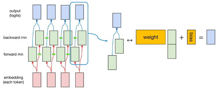
• 이 이미지에서는 시퀀스 -> (Tokenization) -> token -> (Embedding layer) -> numeric vector로 변환한 후, forward RNN, backward RNN이 각각 읽고 각 RNN의 hidden state를 합치게 된다.
  => 정확히는 forward RNN의 hidden state와 backward RNN의 hidden state를 이미지 우측과 같이 Concatenate 방식으로 합쳐서 새로운 벡터를 만들고, 이를 weight와 bias를 활용하여 목적에 맞게 모델링하는 방식이다.
  => 이때 weight와 bias는 모든 토큰의 hidden state에 대해서 동일하게 적용된다.

• *Concatenate : 여러 배열을 특정 축 방향으로 붙여서 하나로 만드는 것.
  ex) [1, 2] Concatenate [3, 4] => [1, 2, 3, 4]

---

구현 예제

• bidirectional RNN은 기존의 Many to Many 방식과 비교해 큰 차이가 없기 때문에 loss func를 계산하는 것도 동일하게 처리된다.
  각 시퀀스의 토큰을 읽고 처리한 결과의 loss들을 계산하고, masking을 활용하여 데이터 간의 길이를 맞추기 위한 pad 토큰을 제외한 실제 데이터의 유효 토큰에 대해 loss를 계산하고 이를 학습에 반영한다.

---

구현 코드

1. 데이터셋 준비

import numpy as np
import tensorflow as tf
from tensorflow import keras
from tensorflow.keras import layers
from tensorflow.keras.models import Sequential
from tensorflow.keras.preprocessing.sequence import pad_sequences
from pprint import pprint
import matplotlib.pyplot as plt

# example data
# 이전 예제와 동일
sentences = [
    ['I', 'feel', 'hungry'],
    ['tensorflow', 'is', 'very', 'difficult'],
    ['tensorflow', 'is', 'a', 'framework', 'for', 'deep', 'learning'],
    ['tensorflow', 'is', 'very', 'fast', 'changing'],
]
pos = [
    ['pronoun', 'verb', 'adjective'],
    ['noun', 'verb', 'adverb', 'adjective'],
    ['noun', 'verb', 'determiner', 'noun', 'preposition', 'adjective', 'noun'],
    ['noun', 'verb', 'adverb', 'adjective', 'verb'],
]

# creating a token dictionary for word
word_list = sum(sentences, [])
word_list = sorted(set(word_list))
word_list = ['<pad>'] + word_list
word2idx = {word: idx for idx, word in enumerate(word_list)}
idx2word = {idx: word for idx, word in enumerate(word_list)}

print(word2idx)
print(idx2word)
print(len(idx2word))

# creating a token dictionary for part of speech
pos_list = sum(pos, [])
pos_list = sorted(set(pos_list))
pos_list = ['<pad>'] + pos_list
pos2idx = {p: idx for idx, p in enumerate(pos_list)}
idx2pos = {idx: p for idx, p in enumerate(pos_list)}

print(pos2idx)
print(idx2pos)
print(len(pos2idx))

=> word dictionary 출력

{'<pad>': 0, 'I': 1, 'a': 2, 'changing': 3, 'deep': 4, 'difficult': 5, 'fast': 6, 'feel': 7, 'for': 8, 'framework': 9, 'hungry': 10, 'is': 11, 'learning': 12, 'tensorflow': 13, 'very': 14}
{0: '<pad>', 1: 'I', 2: 'a', 3: 'changing', 4: 'deep', 5: 'difficult', 6: 'fast', 7: 'feel', 8: 'for', 9: 'framework', 10: 'hungry', 11: 'is', 12: 'learning', 13: 'tensorflow', 14: 'very'}
15

=> pos dictionary 출력

{'<pad>': 0, 'adjective': 1, 'adverb': 2, 'determiner': 3, 'noun': 4, 'preposition': 5, 'pronoun': 6, 'verb': 7}
{0: '<pad>', 1: 'adjective', 2: 'adverb', 3: 'determiner', 4: 'noun', 5: 'preposition', 6: 'pronoun', 7: 'verb'}
8

# converting sequence of tokens to sequence of indices
max_sequence = 10
x_data = list(map(lambda sentence: [word2idx.get(token) for token in sentence], sentences))
y_data = list(map(lambda sentence: [pos2idx.get(token) for token in sentence], pos))

# padding the sequence of indices
x_data = pad_sequences(sequences=x_data, maxlen=max_sequence, padding='post')
x_data_mask = ((x_data != 0) * 1).astype(np.float32)
x_data_len = list(map(lambda sentence: len(sentence), sentences))

y_data = pad_sequences(sequences=y_data, maxlen=max_sequence, padding='post')

# checking data
print(x_data, x_data_len)
print(x_data_mask)
print(y_data)

=> 중간 출력

[[ 1  7 10  0  0  0  0  0  0  0]
 [13 11 14  5  0  0  0  0  0  0]
 [13 11  2  9  8  4 12  0  0  0]
 [13 11 14  6  3  0  0  0  0  0]] [3, 4, 7, 5]
[[1. 1. 1. 0. 0. 0. 0. 0. 0. 0.]
 [1. 1. 1. 1. 0. 0. 0. 0. 0. 0.]
 [1. 1. 1. 1. 1. 1. 1. 0. 0. 0.]
 [1. 1. 1. 1. 1. 0. 0. 0. 0. 0.]]
[[6 7 1 0 0 0 0 0 0 0]
 [4 7 2 1 0 0 0 0 0 0]
 [4 7 3 4 5 1 4 0 0 0]
 [4 7 2 1 7 0 0 0 0 0]]

---

2. 모델 생성

# creating bidirectional rnn for "many to many" sequence tagging
num_classes = len(pos2idx)
hidden_dim = 10

input_dim = len(word2idx)
output_dim = len(word2idx)
one_hot = np.eye(len(word2idx))

model = Sequential()
model.add(layers.InputLayer(input_shape=(max_sequence,)))
model.add(
    layers.Embedding(
        input_dim=input_dim,
        output_dim=output_dim,
        mask_zero=True,
        trainable=False,
        input_length=max_sequence,
        embeddings_initializer=keras.initializers.Constant(one_hot),
    )
)

# 기존 예제에서 Bidirectional만 추가하면 Bidirectional RNN이 된다.
model.add(layers.Bidirectional(layers.SimpleRNN(units=hidden_dim, return_sequences=True)))
model.add(layers.TimeDistributed(layers.Dense(units=num_classes)))

model.summary()

=> 중간 결과

Layer (type)	Output Shape	Param #
embedding (Embedding)	(None, 10, 15)	225
bidirectional (Bidirectional)	(None, 10, 20)	520
time_distributed (TimeDistributed)	(None, 10, 8)	168

항목	값
Total params	913
Trainable params	688
Non-trainable params	225

---

3. 모델 학습

# creating loss function
# 토큰별 loss를 얻기 위해 reduction을 NONE으로 둔다.
loss_obj = tf.keras.losses.SparseCategoricalCrossentropy(
    from_logits=True,
    reduction=tf.keras.losses.Reduction.NONE,
)

def loss_fn(model, x, y, x_len, max_sequence):
    logits = model(x, training=True)  # (batch, time, num_classes)

    # 토큰별 loss: (batch, time)
    per_token_loss = loss_obj(y_true=y, y_pred=logits)

    # pad 제외용 masking: (batch, time)
    masking = tf.sequence_mask(x_len, maxlen=max_sequence, dtype=tf.float32)

    # pad 위치 loss=0
    per_token_loss = per_token_loss * masking

    # 샘플별 평균 loss
    valid_time_step = tf.cast(x_len, dtype=tf.float32)
    loss_per_sample = tf.reduce_sum(per_token_loss, axis=-1) / valid_time_step

    # 미니배치 평균
    sequence_loss = tf.reduce_mean(loss_per_sample)
    return sequence_loss

# creating an optimizer
lr = 0.1
epochs = 30
batch_size = 2
opt = tf.keras.optimizers.Adam(learning_rate=lr)

# generating data pipeline
tr_dataset = tf.data.Dataset.from_tensor_slices((x_data, y_data, x_data_len))
tr_dataset = tr_dataset.shuffle(buffer_size=4)
tr_dataset = tr_dataset.batch(batch_size=batch_size)

print(tr_dataset)
# <BatchDataset shapes: ((?, 10), (?, 10), (?,)), types: (tf.int32, tf.int32, tf.int32)>

# training
tr_loss_hist = []

for epoch in range(epochs):
    avg_tr_loss = 0.0
    tr_step = 0

    for x_mb, y_mb, x_mb_len in tr_dataset:
        with tf.GradientTape() as tape:
            tr_loss = loss_fn(model, x=x_mb, y=y_mb, x_len=x_mb_len, max_sequence=max_sequence)


        grads = tape.gradient(target=tr_loss, sources=model.trainable_variables)
        opt.apply_gradients(grads_and_vars=zip(grads, model.trainable_variables))

        avg_tr_loss += float(tr_loss)
        tr_step += 1

    avg_tr_loss /= tr_step
    tr_loss_hist.append(avg_tr_loss)

    if (epoch + 1) % 5 == 0:
        print('epoch : {:3}, tr_loss : {:.3f}'.format(epoch + 1, avg_tr_loss))

=> 결과 (예시)
epoch : 5, tr_loss : 0.052
epoch : 10, tr_loss : 0.002
epoch : 15, tr_loss : 0.000
epoch : 20, tr_loss : 0.000
epoch : 25, tr_loss : 0.000
epoch : 30, tr_loss : 0.000

---

4. 정확도 확인

yhat = model.predict(x_data, verbose=0)
yhat = np.argmax(yhat, axis=-1) * x_data_mask

pprint(list(map(lambda row: [idx2pos.get(elm) for elm in row], yhat.astype(np.int32).tolist())), width=120)
pprint(pos)

plt.plot(tr_loss_hist)
plt.show()

=> 결과 확인 (예시)

[['pronoun', 'verb', 'adjective', '<pad>', '<pad>', '<pad>', '<pad>', '<pad>', '<pad>', '<pad>'],
 ['noun', 'verb', 'adverb', 'adjective', '<pad>', '<pad>', '<pad>', '<pad>', '<pad>', '<pad>'],
 ['noun', 'verb', 'determiner', 'noun', 'preposition', 'adjective', 'noun', '<pad>', '<pad>', '<pad>'],
 ['noun', 'verb', 'adverb', 'adjective', 'verb', '<pad>', '<pad>', '<pad>', '<pad>', '<pad>']]
[['pronoun', 'verb', 'adjective'],
 ['noun', 'verb', 'adverb', 'adjective'],
 ['noun', 'verb', 'determiner', 'noun', 'preposition', 'adjective', 'noun'],
 ['noun', 'verb', 'adverb', 'adjective', 'verb']]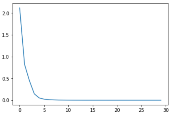

---

모두를 위한 딥러닝 강좌 2
https://www.youtube.com/watch?v=7eldOrjQVi0&list=PLQ28Nx3M4Jrguyuwg4xe9d9t2XE639e5C