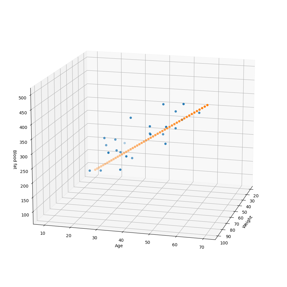
머신러닝이란?
머신러닝은 명시적으로 프로그래밍하지 않고도 컴퓨터에 학습할 수 있는 능력을 부여하는 학문
과거 데이터로부터 얻은 경험이 쌓여 감에따라 주어진 태스크의 성능이 점점 좋아질 때 컴퓨터 프로그램은 경험으로부터 학습한다고 할 수 있음
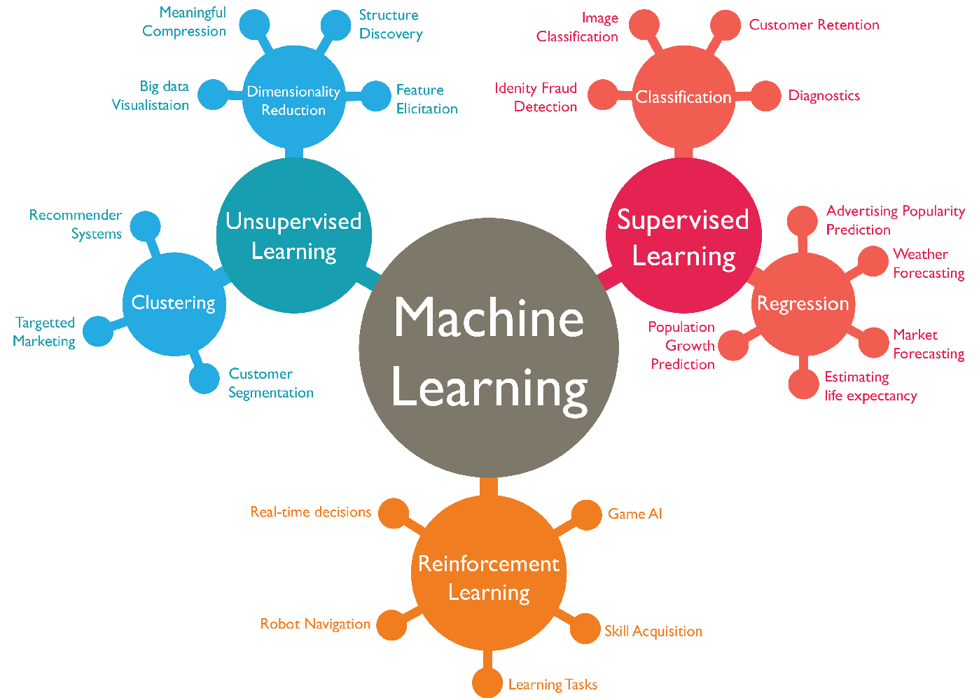
이미지 출처 : Big data and machine learning for Businesses
데이터 관찰
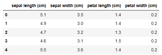
데이터 : iris
from sklearn.datasets import load_iris
iris = load_iris()
iris.keys()
dict_keys(['data', 'target', 'frame', 'target_names', 'DESCR', 'feature_names', 'filename', 'data_module'])
iris 데이터 설명
print(iris['DESCR']).. _iris_dataset:
Iris plants dataset
--------------------
**Data Set Characteristics:**
:Number of Instances: 150 (50 in each of three classes)
:Number of Attributes: 4 numeric, predictive attributes and the class
:Attribute Information:
- sepal length in cm
- sepal width in cm
- petal length in cm
- petal width in cm
- class:
- Iris-Setosa
- Iris-Versicolour
- Iris-Virginica
:Summary Statistics:
============== ==== ==== ======= ===== ====================
Min Max Mean SD Class Correlation
============== ==== ==== ======= ===== ====================
sepal length: 4.3 7.9 5.84 0.83 0.7826
sepal width: 2.0 4.4 3.05 0.43 -0.4194
petal length: 1.0 6.9 3.76 1.76 0.9490 (high!)
petal width: 0.1 2.5 1.20 0.76 0.9565 (high!)
============== ==== ==== ======= ===== ====================
:Missing Attribute Values: None
:Class Distribution: 33.3% for each of 3 classes.
:Creator: R.A. Fisher
:Donor: Michael Marshall (MARSHALL%PLU@io.arc.nasa.gov)
:Date: July, 1988
The famous Iris database, first used by Sir R.A. Fisher. The dataset is taken
from Fisher's paper. Note that it's the same as in R, but not as in the UCI
Machine Learning Repository, which has two wrong data points.
This is perhaps the best known database to be found in the
pattern recognition literature. Fisher's paper is a classic in the field and
is referenced frequently to this day. (See Duda & Hart, for example.) The
data set contains 3 classes of 50 instances each, where each class refers to a
type of iris plant. One class is linearly separable from the other 2; the
latter are NOT linearly separable from each other.
.. topic:: References
- Fisher, R.A. "The use of multiple measurements in taxonomic problems"
Annual Eugenics, 7, Part II, 179-188 (1936); also in "Contributions to
Mathematical Statistics" (John Wiley, NY, 1950).
- Duda, R.O., & Hart, P.E. (1973) Pattern Classification and Scene Analysis.
(Q327.D83) John Wiley & Sons. ISBN 0-471-22361-1. See page 218.
- Dasarathy, B.V. (1980) "Nosing Around the Neighborhood: A New System
Structure and Classification Rule for Recognition in Partially Exposed
Environments". IEEE Transactions on Pattern Analysis and Machine
Intelligence, Vol. PAMI-2, No. 1, 67-71.
- Gates, G.W. (1972) "The Reduced Nearest Neighbor Rule". IEEE Transactions
on Information Theory, May 1972, 431-433.
- See also: 1988 MLC Proceedings, 54-64. Cheeseman et al"s AUTOCLASS II
conceptual clustering system finds 3 classes in the data.
- Many, many more ...데이터 분석 목적 : petal과 sepal의 length, width로 품종을 구분
import pandas as pd

iris_pd=pd.DataFrame(iris.data, columns=iris.feature_names)
iris_pd.head()
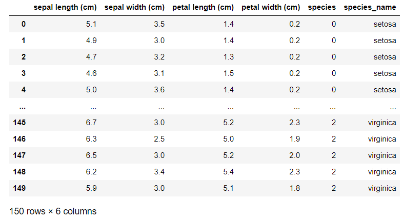
iris_pd['species'] = iris.target
iris_pd['species_name']=iris_pd['species'].apply(lambda x :'setosa' if x==0 else 'versicolor' if x==1 else 'virginica')
iris_pd
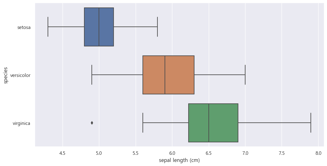
시각화
plt.figure(figsize=(12,6))
sns.boxplot(x='sepal length (cm)', y='species_name', data = iris_pd, orient='h');
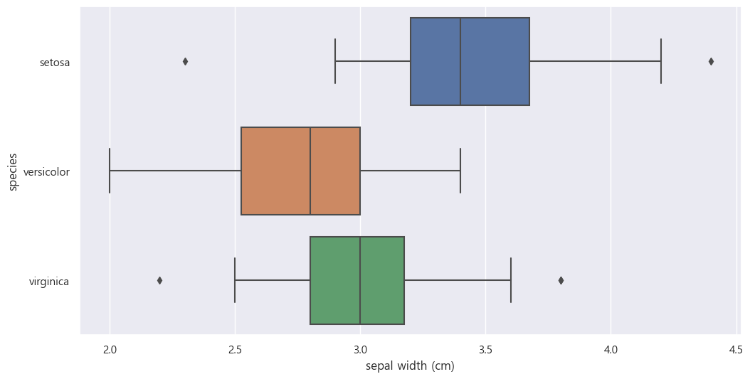
plt.figure(figsize=(12,6))
sns.boxplot(x='sepal width (cm)', y='species_name', data = iris_pd, orient='h');
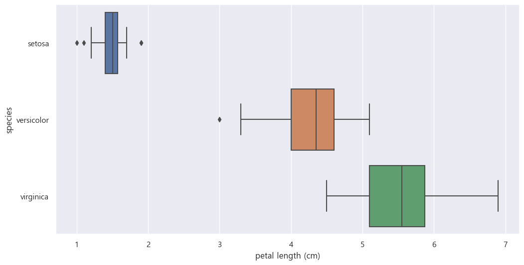
plt.figure(figsize=(12,6))
sns.boxplot(x='petal length (cm)', y='species_name', data = iris_pd, orient='h');
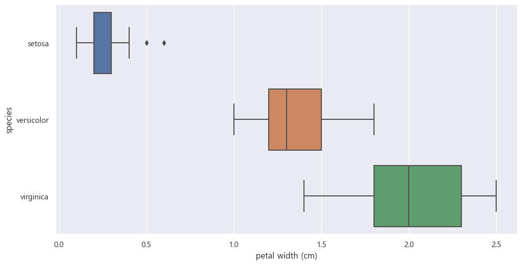
plt.figure(figsize=(12,6))
sns.boxplot(x='petal length (cm)', y='species_name', data = iris_pd, orient='h');
sns.pairplot(iris_pd, hue='species_name')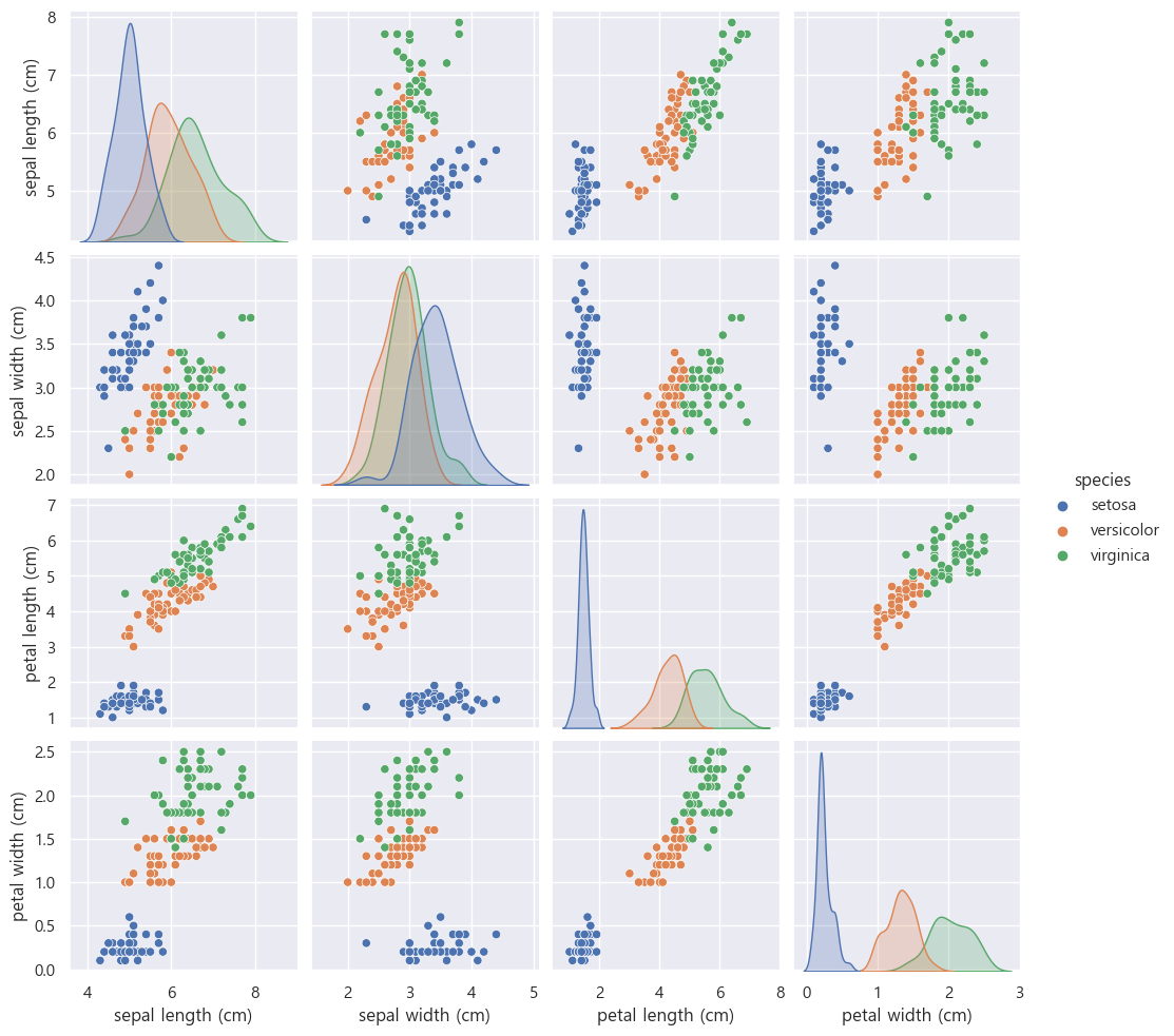
sns.pairplot(iris_pd, hue='species')petal 의 length와 width를 가지고도 iris의 종류를 대략 구분 가능하다.
- 대략 petal length가 2cm보다 작고 petal width가 1cm 이하이면 setosa이다
- 대략 petal length가 3dm 이상 5cm 이하이고 petal width 1.7이하이면 versicolor이다
- 대략 petal length가 5cm 이상이고 petal width 1.7이상이면 virginica이다
sns.scatterplot(iris_pd, x='petal width (cm)', y='petal length (cm)', hue='species_name')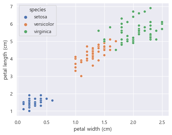
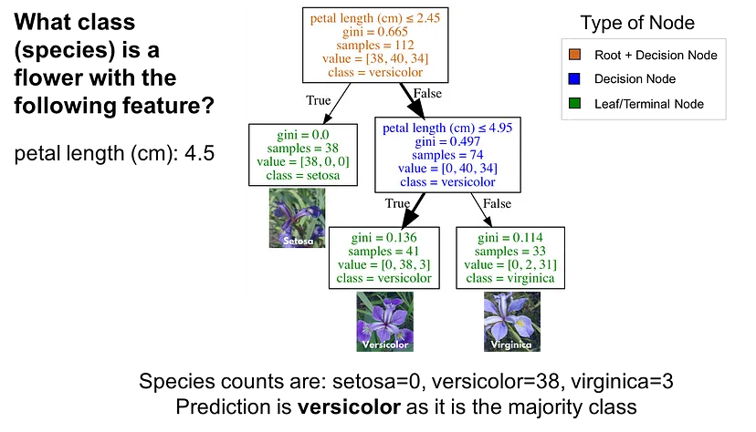
의사결정나무(Decision Tree)
의사결정나무는 데이터를 분석하여 이들 사이에 존재하는 패턴을 예측 가능한 규칙들의 조합으로 나타내며, 그 모양이 ‘나무’와 같다고 해서 의사결정나무라 한다.
Visualizing Decision Trees with Python (Scikit-learn, Graphviz, Matplotlib)
Decision Tree 분할 기준 (Split Criterion)
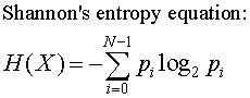
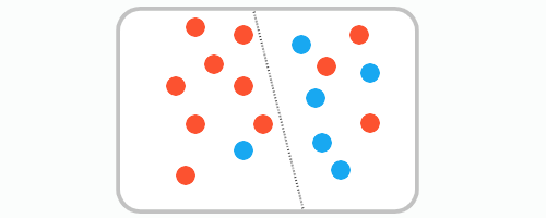
정보 엔트로피
entropy : 얼마만큼의 정보를 담고 있는가? 또한 무질서도(disorder)를 의미, 불확실성(uncertainty)를 나타내기도 함

이미지 출처 : Understanding Entropy
p는 해당 데이터가 해당 클래스에 속할 확률이고 위 식을 그려보면 다음과 같다.
어떤 확률 분포로 일어나는 사건을 표현하는 데 필요한 정보의 양이며 이 값이 커질수로 확률 분포의 불확실성이 커지며 결과에 대한 예측이 어려워짐
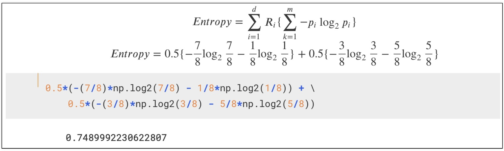
엔트로피 계산
Scikit Learn
파이썬에서 가장 유명한 기계 학습 오픈 소스 라이브러리
fetal 값에 따른 target 학습
from sklearn.tree import DecisionTreeClassifier

iris_tree= DecisionTreeClassifier()
#fetal 값만 가져옴
iris_tree.fit(iris.data[:,2:], iris.target)
fetal 값을 가지고 종류 예측
from sklearn.metrics import accuracy_score

y_pred_tr = iris_tree.predict(iris.data[:,2:])
y_pred_tr
array([0, 0, 0, 0, 0, 0, 0, 0, 0, 0, 0, 0, 0, 0, 0, 0, 0, 0, 0, 0, 0, 0,
0, 0, 0, 0, 0, 0, 0, 0, 0, 0, 0, 0, 0, 0, 0, 0, 0, 0, 0, 0, 0, 0,
0, 0, 0, 0, 0, 0, 1, 1, 1, 1, 1, 1, 1, 1, 1, 1, 1, 1, 1, 1, 1, 1,
1, 1, 1, 1, 2, 1, 1, 1, 1, 1, 1, 1, 1, 1, 1, 1, 1, 1, 1, 1, 1, 1,
1, 1, 1, 1, 1, 1, 1, 1, 1, 1, 1, 1, 2, 2, 2, 2, 2, 2, 2, 2, 2, 2,
2, 2, 2, 2, 2, 2, 2, 2, 2, 2, 2, 2, 2, 2, 2, 2, 2, 2, 2, 2, 2, 2,
2, 2, 2, 2, 2, 2, 2, 2, 2, 2, 2, 2, 2, 2, 2, 2, 2, 2])예측값 비교
iris.target
array([0, 0, 0, 0, 0, 0, 0, 0, 0, 0, 0, 0, 0, 0, 0, 0, 0, 0, 0, 0, 0, 0,
       0, 0, 0, 0, 0, 0, 0, 0, 0, 0, 0, 0, 0, 0, 0, 0, 0, 0, 0, 0, 0, 0,
       0, 0, 0, 0, 0, 0, 1, 1, 1, 1, 1, 1, 1, 1, 1, 1, 1, 1, 1, 1, 1, 1,
       1, 1, 1, 1, 1, 1, 1, 1, 1, 1, 1, 1, 1, 1, 1, 1, 1, 1, 1, 1, 1, 1,
       1, 1, 1, 1, 1, 1, 1, 1, 1, 1, 1, 1, 2, 2, 2, 2, 2, 2, 2, 2, 2, 2,
       2, 2, 2, 2, 2, 2, 2, 2, 2, 2, 2, 2, 2, 2, 2, 2, 2, 2, 2, 2, 2, 2,
       2, 2, 2, 2, 2, 2, 2, 2, 2, 2, 2, 2, 2, 2, 2, 2, 2, 2])
# 예측 정확도
accuracy_score(iris.target, y_pred_tr)
0.9933333333333333

개발하고싶은사람