이 논문은 Anomaly Detection의 Deep learning을 이용한 방법들을 Survey한 내용을 담고 있다.'
앞 부분은 Anomaly Detection의 역사나, 다른 Survey 논문과의 차이 등을 담고 있어 생략한다.

ANOMALOUS NODE DETECTION(ANOS ND)

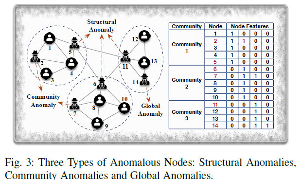
node anomaly엔 크게 3종류가 있다.

• Global anomalies
  - node의 attributes만 고려하는 anomaly이다.
  • 전체 그래프에서 다른 노드들과 다른 attributes를 가지고 있는 node를 찾는다.
• Structural anomalies
  - 그래프의 structure만 고려하는 anomaly이다.
  • 비정상적인 노드는 다른 connection pattern을 가지고 있다.
• Community anomalies
  - 둘을 모두 고려한다.
  - 같은 커뮤니티의 node와 다른 attributes를 가지고 있는 node를 찾는다.
  위의 그림을 보면 쉽게 이해할 수 있다.

ANOS ND on Plain Graphs(No Attributes)

• Network Representation Based Techniques
  이 방법은 그래프의 구조를 embedded vector space로 변환해 처리하는 방법이다.
  예를 들어 graph partitioning algorithm(METIS)를 이용해 그래프를 d개의 커뮤니티로 나눈 후에, embedding으로 각 노드와 커뮤니티 간의 정보를 잡아낸다.
  node i의 embedding을 $Z_i=\{z_i^1, z_i^2,...,z_i^d\}$로 둬서 커뮤니티 c에 속한다면 $z_i^c=\frac{1}{\sqrt{2}}$로 두고 그렇지 않으면 0으로 둔다. 직접 연결된 node들은 비슷한 embedding을 가지고 그렇지 않다면 다른 embedding을 가지도록 만든다.
  이를 통해 node i와 커뮤니티와의 관계를 아래와 같이 수치화할 수 있다.
  $\overline{NB(i)}=\{y_i^1,...,y_i^d\}=\displaystyle\sum_{j\in \mathcal{N}(i)}(1-\|Z_i-Z_j\|)\cdot Z_j$
  만약 node i와 커뮤니티 c와 많은 link가 존재하면 $y_i^c$의 값이 클 것이다.
  마지막으로 anomalousness score를 매긴다.
  $AScore(i)=\displaystyle\sum^d_{k=1}\frac{y_i^k}{y_i^*},\ y_i^*=max\{y_i^1,...,y_i^d\}$
  만약 AScore가 threshold를 넘어서면 이를 Anomaly로 간주한다.

현재는 Deepwalk, Node2Vec, LINE등의 여러 Representation 기반의 방법들이 존재한다. 이 방법의 장점은 쉽게 기존의 anomaly detection 알고리즘과 짝지어 사용할 수 있다는 것이다.

• Reinforcement Learning Based Techniques
  Reinforcement Learning이 큰 성공을 이루며 Graph Network에도 이를 적용하기 위한 여러 시도가 있었다.
  Selective harvesting을 위해 제시된 NAC 모델은 RL과 embedding을 합쳐서 사용한다.
  이 방법은 부분적으로 관찰된 node와 edge를 seed network로 삼는다.
  이후 seed network에서 시작해서 reinforcement learning을 통해 node selection plan을 만들어 관찰되지 않은 부분에서의 anomalous node를 찾아낼 수 있다.
  이는 reward selection plan을 labeled anomalies를 higher gains로 선택함으로써 가능하다.

ANOS ND on Attributed Graphs

실제 네트워크는 관계로만 생기는 것이 아닌 각 node의 attribute가 존재하므로 이를 이용해야 더 많은 hidden anomaly를 찾을 수 있다.

• Deep NN Based Techniques
  
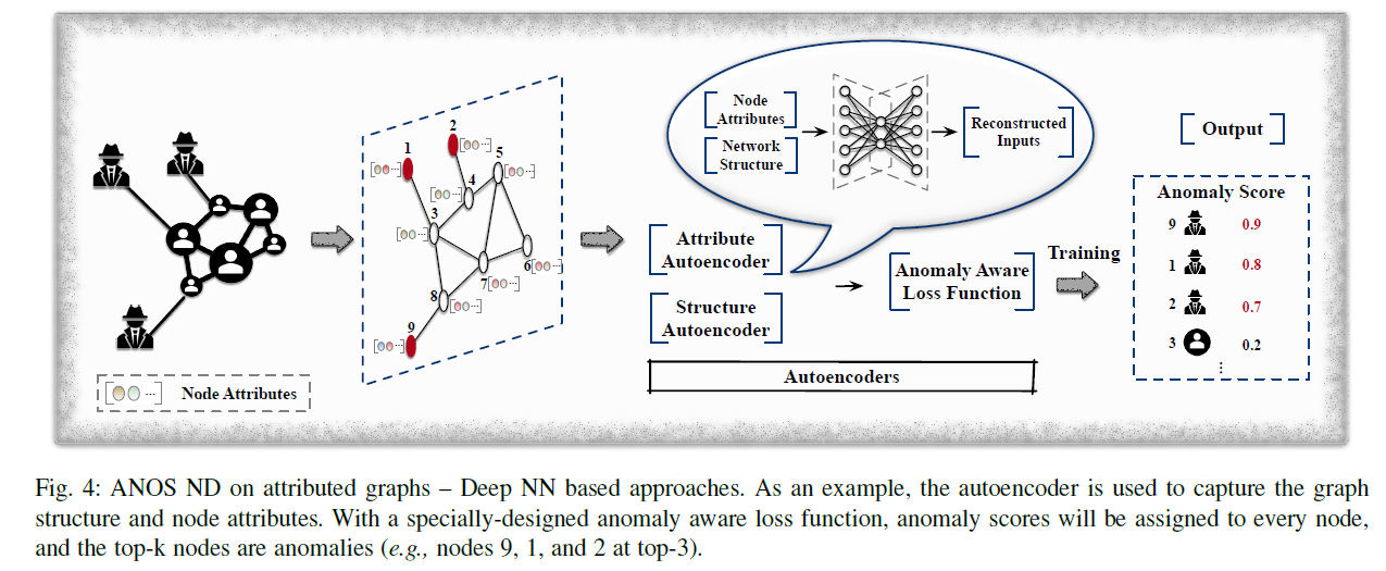
  autoencoder와 DNN을 이용하는 모델은 data representation을 학습하는데 탁월하다.
  예를 들어 global anomalies, structural anomalies, community anomalies를 탐지하기 위한 unsupervised 모델인 DONE이 있다.
  이 모델은 3가지 anomaly score를 매긴다.

1. $o_i^a$: 다른 커뮤니티의 노드와 비슷한 attributes를 가진다.

2. $o_i^s$: 다른 커뮤니티와 연결된다.

3. $o_i^{com}$: structural 하게는 한 커뮤니티에 속하지만 다른 커뮤니티의 attributes 패턴을 가진다.
   어느 노드가 이 중 하나라도 높은 점수를 가진다면 anomalous로 판단된다.

   score를 계산하기 위해 DONE은 structural autuencoder와 attribute autoencoder를 이용한다.
   둘 모두 reconstruction error를 최소화하고 connected nodes가 비슷한 representation을 가지도록 한다.
   학습을 위해 DONE은 fine term을 가진 loss function을 만들었다.
   structure reconstruction error와 attribute reconstruction error는 아래와 같이 계산된다.
   $\mathcal{L}^{Recs}_{str}=\frac{1}{N}\displaystyle\sum_{i=1}^N log(\frac{1}{o_i^s})\|t_i-\hat t_i\|^2_2,\ \mathcal{L}^{Recs}_{attr}=\frac{1}{N}\displaystyle\sum_{i=1}^N log(\frac{1}{o_i^a})\|x_i-\hat x_i\|^2_2$
   N은 node의 개수이고, $t_i, x_i$는 각각 structure, attributes of node i이다.
   connected nodes가 비슷한 representation을 가지게 하기 위한 homophily loss는 다음과 같다.
   $\mathcal{L}^{Hom}_{str}=\frac{1}{N}\displaystyle\sum_{i=1}^N log(\frac{1}{o_i^s})\frac{1}{|N(i)|}\sum_{j \in N(i)}\|h_i^s-h_j^s\|^2_2$
   $\mathcal{L}^{Hom}_{attr}=\frac{1}{N}\displaystyle\sum_{i=1}^N log(\frac{1}{o_i^a})\frac{1}{|N(i)|}\sum_{j \in N(i)}\|h_i^a-h_j^a\|^2_2$
   $h_i^s, h_i^a$는 각각 structure AE, attribute AE에서 학습된 latent representation이다.
   $\mathcal{L}^{Com}=\frac{1}{N}\displaystyle\sum_{i=1}^N log(\frac{1}{o_i^{com}})\|h_i^s-h_i^a\|^2_2$
   com loss는 graph structure와 node attributes가 서로를 보충하도록 해준다.
   전체 loss는 이들의 sum으로 이루어지고, top-k 노드가 anomaly node로 지정된다.

• GNN Based Techniques
  link prediction, node classification, recommendation 등에서 많이 사용되는 GCN 모델은 anomaly detection에도 이용된다.
  DOMINANT 모델은 graph convolutional encoder, structure reconstruction decoder, attribute reconstructure decoder를 이용한 모델이다.
  graph convolutional encoder는 GCN layer 여러 개를 거쳐 node embeddings를 만들고, 각각 structure, attribute reconstructure decoder는 embedding을 이용해 network structure와 node attribute matrix를 재구성한다.
  $\mathcal{L}_{DOMINANT}=(1-\alpha)\mathcal{R}_S+\alpha \mathcal{R}_A=(1-\alpha)\|A-\hat A\|^2_F + \alpha \|X-\hat X|^2_F$
  위의 loss function을 이용해 학습을 진행하고, 아래의 식을 이용해 각 node의 anomaly score가 계산된다.
  $score(i)=(1-\alpha)\|a_i-\hat a_i\|_2 + \alpha \|x_i-\hat x_i\|_2$
  anomaly score을 topk하여 anomalies를 결정한다. 이후 성능을 더 올리기 위해 node attributes를 더 다양한 view에서 관찰하게 되었는데, 예를 들어 온라인 커뮤니티에서 demographic information(인구통계정보)와 포스팅된 글을 다른 뷰로 봐서 각각이 personal information과 social activities를 나타내도록 하는 것이다. 이를 통해 하나의 view로 정상으로 판단되더라도 다른 view에서 anomaly로 판단될 수 있다.
  ALARM 방법은 여러개의 GCN을 이용해 multiple views를 encode한다. 이후 weighted aggregation을 통해 node representation을 생성한다.
  $\mathcal{L}_{ALARM}=\displaystyle\sum_{i=1}^{n}\sum_{j=1}^{n}- [\gamma A_{ij}log \hat A_{ij} + (1-A_{ij})log(1-\hat A_{ij})] + \|X - \tilde X\|_2^F$
  ALARM은 위와 같은 loss function으로 학습을 진행하고, DOMINANT와 같은 방법으로 anomaly score을 매긴다.
  
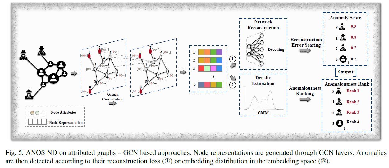
  SpecAE는 Gaussian Mixture Model을 이용해 anomalies를 찾는다.
  위의 그림과 같이 graph convolutional encoder를 이용해 node representation을 만들어내고 deconvolutional decoder를 통해 attributes를 reconstruct한다.
  global, community anomalies는 다른 노드와 다른 attribute patterns를 가지고 있으므로 GMM 내에서 정상적인 노드들보다 더 낮은 energy를 가진다. 이를 통해 topk node with lowest probabilities는 anomaly로 판단된다.
  이 외에 Fdgar, GraphRfi(anomaly detection과 recommendation을 합친 모델) 등이 GCN 기반의 모델이다.
  
• Reinforcement Learning Based Techniques
  GraphUCB 모델은 NAC과 다르게 attribute information도 이용하여 contextual multi-armed bandit technology 를 이용해 학습된다.

ANOS ND on Dynamic Graphs

실제 데이터들은 노드 관의 관계나 특성이 계속 바뀌므로 dynamic graphs로 모델링 될 수 있다. dynamic graph는 structural information과 node attributes 외에 temporal signals를 가지고 있다.
이런 데이터는 데이터의 양을 크게 증가시키므로 anomaly detection을 어렵게 만들지만, 더 많은 detail을 제공해 줄 수 있다.
예를 들어 어느 한 snapshot에선 정상으로 보이는 anomalies들도 시간에 따라 바뀌는 모습을 보면 찾을 수 있을 수 있다.

• Network Representation Based Techniques
  NetWalk 모델은 plain graph에서 autoencoder를 이용해 첫 그래프에서 representation을 학습하고 업데이트를 해 나가는 방식이다.
  anomaly를 탐지하기 위해 NetWalk는 k-means를 통해 현재 time stamp를 여러 cluster로 그룹화한다. anomaly score는 k cluster와의 closest distance를 이용해 계산된다.
  그래프가 변해가면서 cluster center과 anomaly score도 재계산된다.
• GAN Based Techniques
  Anomaly detection은 ground truth data의 부족으로 고통받는데, 이를 해결하기 위해 GAN을 통해 simulated data를 생성할 수 있다.
  이를 이용하면 정상적인 유저의 attribute 만을 이용해 문제를 해결할 수 있다. 이는 정상적인 행동 패턴을 학습하여 확연히 다르게 행동하는 anomaly를 포착함으로써 할 수 있다.
  OCAN은 정상적인 유저의 content feature와 historical social behavior를 LSTM based autoencoder를 이용해 latent space로 추출한다.
  이러면 정상적인 유저와 malicious 유저는 feature space의 다른 공간에 위치하게 된다.
  다음으로 adversarial network의 generator와 distriminator를 학습한다. 이를 통해 generator는 정상 유저의 low density areas의 data를 생성하게 되고, discriminator는 이를 정상유저의 data와 구별할 수 있게 된다. 학습을 통해 discriminator는 정상 유저의 region을 구별할 수 있게 된다.

NetWalk와 OCAN은 각자의 역할을 잘 해나가지만 각각 structure과 attribute만 고려하고 있다는 한계점이 있다. static graph에서는 둘 모두를 고려한 모델이 성공적으로 만들어지고 있다는 것을 생각했을 때, dynamic graph에서도 둘을 모두 고려한다면 더 좋은 성능을 낼 것이라 기대한다.

ANOMALOUS EDGE DETECTION(ANOS ED)

ANOS ED는 비정상적인 link를 찾는데 집중한다. 예를 들어 정상적인 유저와 비정상적인 유저의 관계를 밝혀내는데 이용될 수 있다.

• Deep NN Based Techniques
  
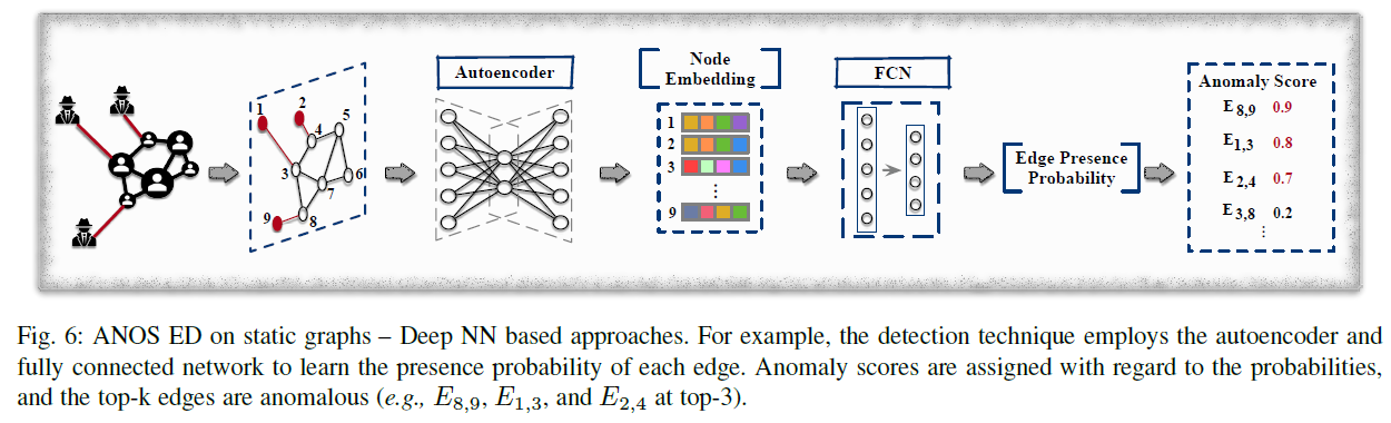
  앞의 경우와 마찬가지로 autoencoder와 Fully Connected Network 등이 이용될 수 있다.
  UGED는 각 노드를 FCN layer를 거쳐서 lower-dimensional vector로 변환한다. 이 후 u 노드와 이웃들의 vector를 mean aggregation하여 node representation을 생성한다. 이를 다른 FCN Layer에 넣어 edge의 확률을 계산한다.
  UGED의 목표는 cross entropy loss를 이용해 실제 존재하는 edge의 prediction을 최대화해서 실제로 존재하는 edge이지만 낮은 prediction을 가지고 있다면 higher score를 가지도록 하는 방식이다.
  

• GCN Based Techniques
  GCN의 문제점은 훈련 데이터에 존재하는 anomalous edges의 존재가 real edge distribution을 학습하는 것을 방해한다는 것이다.
  이를 해결하기 위해 node embedding은 anomalous edge의 negative impact가 완화되도록 만들어져야한다.
  AANE 모델은 embedding과 detection results를 순회하면서 업데이트 하는 방식으로 이를 해결한다.
  각 training iteration에 AANE는 GCN layer를 거치며 node embedding Z를 만들고 indicator matrix I를 학습한다.
  $I$는 $I_{uv}=1$ if $\hat A_{uv} < mean_{v' \in N_u}A_{uv'}-\mu \cdot std_{v' \in N_u}\hat A_{uv'}$ otherwise 0
  로 계산된다.
  $\hat A_{uv}$는 u와 v의 embedding의 hyperbolic tangent로 계산된 predicted link probability이고, $\mu$는 predefined threshold이다.
  이를 통해 edge uv는 node u와 관련된 모든 링크의 average보다 probability가 threshold 만큼 작을 때 anomaly로 판정된다.
  AANE의 loss는 두 가지(anomaly-aware loss $\mathcal{L}_{aal}$, adjusting fitting loss $\mathcal{L}_{afl}$)로 구성된다.
  $\mathcal{L}_{aal}=\displaystyle\sqrt{\sum_{u \in V} \sum_{v \in N(u)} ((1-\hat A^2_{uv})(1 - I_{uv}) + \hat A^2_{uv}I_{uv})}$
  $\mathcal{L}_{afl}=\|B-\hat A\|_2^2$
  B는 input adjacency matrix에서 predicted anomaly를 모두 없앤 값이다.

• Network Representation Based Techniques
  몇 가지 방법이 제시되어 있고 나쁘지 않은 성능을 보여준다.

ANOS ED on Dynamic Graphs

Dynamic graph에서 edge는 시간에 따라 생겨나고 사라진다.

• Network Representation Based Techniques
  dynamic graph structure information을 edge representation으로 나타내서 기존의 anomaly detection 기법을 이용해 비정상적인 edge를 검출하는 것이 가능하다. 그러나 dynamic graph에선 edge representation을 생성하고 업데이트 하는 것이 까다로운데, 이미 ANOS ND의 NetWalk에서 anomalous edge를 검출하는 것이 가능하다.
  NetWalk는 edge를 node embedding을 이용해 shared latent space로 encode할 수 있고, 이후 distance based anomaly detection을 이용해 latent space의 closest edge-cluster center와의 거리로 anomaly를 밝혀낼 수 있다.
  NetWalk는 Hadamard product(element-wise product)를 이용해
  $z_{u,v}=z_u \odot z_v$ 를 계산하고, node나 edge representation이 업데이트 될 때마다 새로 계산한다.
  edge cluster와 가장 먼 top k edge는 anomaly로 간주된다.
• GCN Based Techniques
  
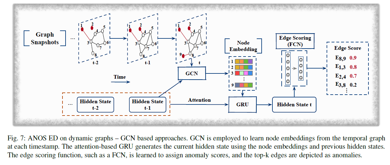
  NetWalk는 효과적이지만 node와 edge struction의 evolving pattern을 고려하지 않는다. 이를 위해 AddGraph는 temporal, structural, attribute information을 합쳐서 고려한다.
  이 모델은 GCN, GRU with attention으로 이루어져 있어 time step 간의 dependencies를 잡아낸다.
  각 time step에서 GCN을 통해 output hidden state $H^{t-1}$을 이용해 node embedding을 만들고 이를 GRU에 넣어 hidden state $H^{t}$를 생성한다.
  $f(u, v, w)=w\cdot \sigma(\beta \cdot (\|a \odot h_u + b \odot h_v\|^2_2 - \mu))$
  로 edge anomaly score를 계산한다. u, v는 인접한 node이고 w는 edge의 weight, a, b는 학습되는 파라미터이고, $\beta, \mu$는 하이퍼 파라미터이다.
  a와 b를 학습하기 위해 아래의 loss function을 이용한다. 존재하는 edge를 정상으로 간주하고 sample된 non-existing edge를 비정상으로 간주한다.
  $\mathcal{L}_{AddGraph}=min\displaystyle\sum_{(u,v,w) \in \epsilon^t}\sum_{(u',v',w') \notin \epsilon^t}max\{0, \gamma + f(u,v,w) - f(u',v',w')\} + \lambda \mathcal{L}_{reg}$

ANOMALOUS SUB-GRAPH DETECTION(ANOS SGD)

실제로는 어떤 유저 그룹이 공모하여 잘못된 리뷰를 올리거나 할 수도 있다. 이런 경우 anomaly는 어떤 sub graph를 형성하게 되는데 ANOS SGD는 이를 찾기 위한 모델이다.
이전과 달리 수상한 sub graph의 각 node와 edge는 정상적일 수 있다. 그러나 이를 모아서 보면 anomaly가 될 수 있다. 이런 점 때문에 ANOS SGD는 ANOS ND나 ANOS ED보다 더 어려운 작업이다.
같은 그룹의 수상한 유저는 vector space에서 가깝게 위치한다는 점으로 학습을 진행할 수 있다.
Shopping network에서 이를 이용해 만들어진 DeepFD는 유저 간의 similiarity $sim_{ij}$를 정의하는데, 이는 전체 제품 중에 이 유저들이 동시에 리뷰한 제품들의 비율(Percentage)을 의미한다.
후에 User representation이 3개의 loss($\mathcal{L}_{res},\mathcal{L}_{sim},\mathcal{L}_{reg}$)를 가진 autoencoder로 학습된다.
다른 loss들은 다른 모델과 거의 같고,
$\mathcal{L}_{sim}=\displaystyle\sum_{i,j=1}^{m}sim_{ij}\cdot\|\widehat{sim}_{ij}-sim_{ij}\|^2_2$
$\widehat{sim}_{ij}$은 user i와 j의 similarity를 RBF kernel나 다른 방법으로 계산한다.
마지막으로 수상한 block들은 DBSCAN을 이용해 감지된다.
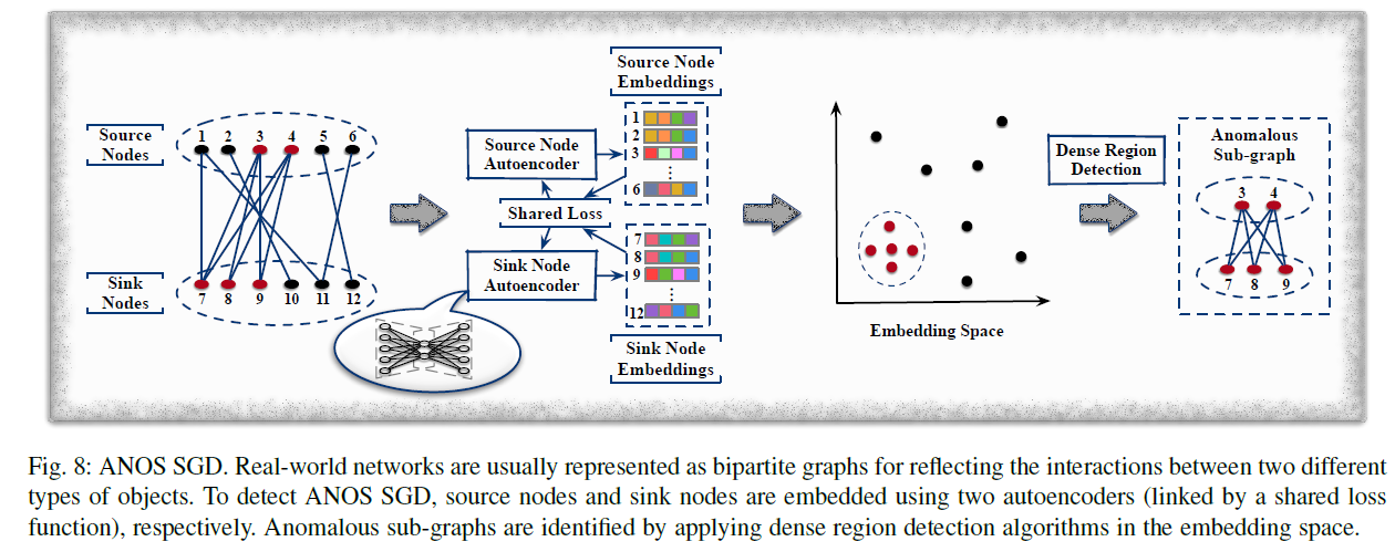
FraudNE 또한 online review network를 이분 그래프로 나타내 dense block detection을 수행한다. DeepFD와 다른 점은 FraudNE는 user와 item을 shared latent space로 encode해서 같은 dense block에 위치하는 user와 item은 비슷한 distribution을 가지도록 하는 것이다.
FraudNE는 source node autoencoder와 sink node autoencoder를 가지고 각각 user representation과 item representation을 학습한다.
$\mathcal{L}_{FraudNE}=\mathcal{L}^{source}_{res}+\mathcal{L}^{sink}_{res}+\alpha\cdot\mathcal{L}_{share}+\alpha\cdot\mathcal{L}_{reg}$

이 loss는 연결된 item과 user가 비슷한 representation을 가지도록 한다.

ANOMALOUS GRAPH DETECTION(ANOS GD)

ANOS GD는 데이터베이스 내의 여러가지 그래프 중에 다른 것들과 확연히 다른 그래프를 찾는 작업이다.
분자, 화학식 구조에서 비정상적인 분자를 찾아내거나, brain graph 중에 brain disorder을 진단하는 등의 작업에 이용될 수 있다.

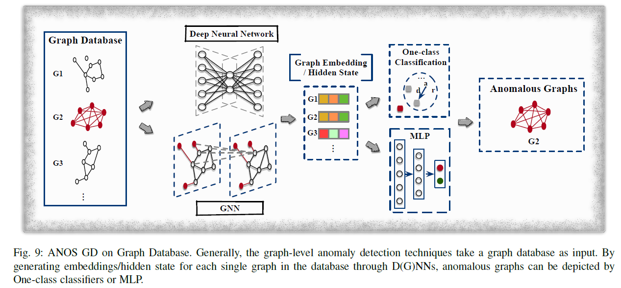
• GNN Based Techniques
  GNN이 ANOS GD에도 이용될 수 있는데, 예를 들어 fake news detection을 만들기 위해, tree구조의 graph를 만들어 root node를 뉴스로 두고, child node를 뉴스와 접촉을 한 user로 둘 수 있다.
  UPFD 모델은 news piece와 user의 embedding을 text embedding 모델을 이용해 각각 추출한다.
  각각 news graph에 대해 latent presentation은 news와 user의 embedding을 concatenate하여 만들고 이를 news의 label과 함께 classifier에 넣어서 fake news로 밝혀진 news graph는 anomaly로 처리하도록 한다.
  또한 다른 예시로 GIN model과 one-class classification(DeepSVDD)을 이용해 end-to-end로 구현할 수 있다. 각 그래프의 embedding은 그래프 내의 node들의 embedding을 mean-pooling해서 만들고 hypersphere에 바깥에 존재하는 그래프를 anomaly로 처리하는 방식이다.
• Network Representation Based Techniques
  graph-level representation technique을 적용하는 것이 가능하다. 이를 이용하면 이 문제는 기존의 outlier detection 문제를 적용하면 끝난다.
  앞의 GNN기반의 end-to-end 모델과 비교했을 때, 이 방법은 two-stage로 나뉘게 된다.
  1. 그래프를 Graph2Vec, FGSD 등을 이용해 shared latent space로 encoding한다.
  2. outlier detector를 이용해 anomaly를 찾는다.
  이 방법의 문제점은 각 stage가 ANOS GD를 위해 디자인 된 것이 아니기 때문에 성능 문제가 있을 수 있다.

ANOS GD on Dynamic Graphs

ANOS ND, ANOS ED on DYNAMIC GRAPHS와 비슷하게 진행된다. GNN, LSTM, autoencoder를 적용할 수 있다.
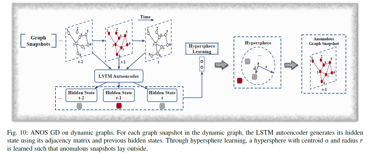
그림에서 묘사한 DeepSphere 모델과 같이 LSTM을 적용해 비정상적인 graph snapshot을 찾는 것이 가능하다.
dynamic graph는 $\{\mathcal{X}_k, k=1,2,3,...\}, \mathcal{X}\in \mathcal{R}^{N\times N\times T}$ 로 묘현될 수 있다.(각 time dimension이 adjacency matrix를 나타낸다.)
DeepSphere는 각 graph snapshot을 LSTM autoencoder를 통해 latent space로 embedding한다.
이후 이를 one-class classification을 통해 분류하여 hypersphere의 밖에 존재하면 anomalous snapshot으로 간주한다.
hypersphere는 아래의 loss로 학습된다.
$\mathcal{L}_h=r^2+\gamma\displaystyle\sum^m_{k=1}\epsilon_k+\frac{1}{m}\sum^m_{k=1}\|z_k-a\|^2$
$z_k$는 latent representation, a는 centroid of hypersphere, r은 radius, $\epsilon_k$는 outlier penalty($\epsilon_k=\|z_k-a\|^2-r^2$)이고 m은 snapshot의 개수, $\gamma$는 하이퍼 파라미터이다. DeepSphere의 전체 loss는 다음과 같다.
$\mathcal{L}=\mathcal{L}_h+\lambda\mathcal{L}_{res}$

그 외

Awesome-Deep-Graph-Anomaly-Detection에 수 많은 모델들과 데이터셋을 정리해 놓았다.
뒤의 Future Directions나 Appendix(Anomaly detection의 어려운 점, 기존의 tradition한 방법 등)에도 유익한 내용이 많이 있으니 읽어보면 좋을 것 같다.