Machine Learning by professor Andrew Ng in Coursera Logistic Regression Model
1) Cost Function
logistic regression에서는 parameter θ θ θ
Linear Regression:
J ( θ ) = 1 m ∑ i = 1 m 1 2 ( h θ ( x ( i ) − y ( i ) ) ) 2 ⏟ cost ( h θ ( x ) , y ) J(\theta)=\frac{1}{m} \sum_{i=1}^{m} \underbrace{ \frac{1}{2} \left(h_\theta(x^{(i)}-y^{(i)} )\right)^2}_{\color{royalblue}{\textrm{cost}\left(h\theta (x) , y\right)}} J ( θ ) = m 1 i = 1 ∑ m cost ( h θ ( x ) , y ) 2 1 ( h θ ( x ( i ) − y ( i ) ) ) 2 하지만 logistic regression에 같은 cost function을 적용하면 non-convex function 이 된다.non-convex function은 경사하강법을 적용해도 최솟값에 도달한다는 보장이 없기 때문이다.
Logistic Regression Cost Function
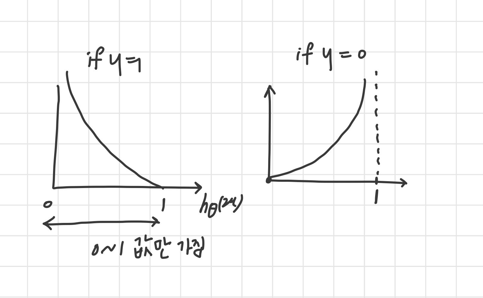
cost ( h θ ( x ) , y ) = { − log ( h θ ( x ) ) if y = 1 − log ( 1 − h θ ( x ) ) if y = 0 \text{cost}\big( h_\theta (x), y \big) = \begin{cases} -\log\big(h_\theta (x)\big) & \text{if } y=1 \\ -\log \big(1-h_\theta (x) \big) & \text{if } y=0 \end{cases} cost ( h θ ( x ) , y ) = { − log ( h θ ( x ) ) − log ( 1 − h θ ( x ) ) if y = 1 if y = 0
cost = 0 if y = 1 and h θ ( x ) = 1 \text{cost}=0 \text{ if } y = 1 \text{ and } h_\theta(x) = 1 cost = 0 if y = 1 and h θ ( x ) = 1 예측을 1로 했고, y가 실제로도 1이면 cost = 0 cost → ∞ as h θ ( x ) → ∞ \text{ cost} \to \infty \text{ as } h_\theta(x) \to \infty cost → ∞ as h θ ( x ) → ∞
2) Simplified Cost Function and Gradient Descent
Logistic Regression Cost Function
Logistic Regression:
J ( θ ) = 1 m ∑ i = 1 m cost ( h θ ( x ( i ) ) , y ( i ) ) J(\theta) = \frac{1}{m} \sum_{i=1}^{m} \text{cost}\left( h_\theta ( x^{(i)}), y^{(i)} \right) J ( θ ) = m 1 i = 1 ∑ m cost ( h θ ( x ( i ) ) , y ( i ) ) w h e r e cost ( h θ ( x ) , y ) = { − log ( h θ ( x ) ) if y = 1 − log ( 1 − h θ ( x ) ) if y = 0 where \text{cost}\left( h_\theta (x), y \right) = \begin{cases} -\log(h_\theta (x)) & \text{if } y=1 \\ -\log(1-h_\theta (x)) & \text{if } y=0 \end{cases} w h e r e cost ( h θ ( x ) , y ) = { − log ( h θ ( x ) ) − log ( 1 − h θ ( x ) ) if y = 1 if y = 0 를 간단하게 나타내면 아래와 같다.
C o s t ( h θ ( x ) , y ) = − y log ( h θ ( x ) ) − ( 1 − y ) log ( 1 − h θ ( x ) ) Cost(h_\theta(x), y) = -y\log(h_\theta(x)) - (1 - y)\log(1 - h_\theta(x)) C o s t ( h θ ( x ) , y ) = − y log ( h θ ( x ) ) − ( 1 − y ) log ( 1 − h θ ( x ) ) 최종 Logistic regression cost function :
J ( θ ) = − 1 m ∑ i = 1 m [ y ( i ) log h θ ( x ) + ( 1 − y ( i ) ) log ( 1 − h θ ( x ) ) ] J(\theta) = - \frac{1}{m} \sum_{i=1}^{m} \left[ y^{(i)} \log h_\theta (x) + (1-y^{(i)}) \log \left( 1-h_\theta (x) \right) \right] J ( θ ) = − m 1 i = 1 ∑ m [ y ( i ) log h θ ( x ) + ( 1 − y ( i ) ) log ( 1 − h θ ( x ) ) ] J ( θ ) J(\theta) J ( θ ) θ \theta θ
R e p e a t { θ j : = θ j − α ∂ ∂ θ j J ( θ ) } ( 모든 θ j 동시에업데이트 ) Repeat \{ \theta_j := \theta_j - \alpha \frac{\partial}{\partial \theta_j} J(\theta) \} (모든 \theta_j 동시에 업데이트) R e p e a t { θ j : = θ j − α ∂ θ j ∂ J ( θ ) } ( 모 든 θ j 동 시 에 업 데 이 트 ) 이때
∂ ∂ θ j J ( θ ) = 1 m ∑ i = 1 m ( h θ ( x ( i ) ) − y ( i ) ) x j ( i ) \frac{\partial}{\partial \theta_j} J(\theta) = \frac{1}{m} \sum_{i=1}^{m} \left( h_\theta(x^{(i)}) - y^{(i)} \right) x_j^{(i)} ∂ θ j ∂ J ( θ ) = m 1 i = 1 ∑ m ( h θ ( x ( i ) ) − y ( i ) ) x j ( i ) linear regression의 gradient descent와 비교 해보면, 식의 형태가 동일 한 것을 알 수 있다.hypothesis 정의 가 서로 다르다.
linear regression :
h θ ( x ) = θ T ( x ) h_\theta(x) = \theta^T(x) h θ ( x ) = θ T ( x ) logistic regression :
h θ ( x ) = 1 1 + e − θ T x h_\theta(x) = \frac{1}{1 + e^{-\theta^Tx}} h θ ( x ) = 1 + e − θ T x 1 linear regression에서 feature scaling을 통해 gradient descent를 더 빠르게 수렴하도록 하기도 했는데 이 방법은 logistic regression에도 적용된다.
3) Advanced Optimization
Optimization algorithm
Gradient Descent
Conjugate gradient
BFGS
LBFGS
1 vs 2, 3, 4
2, 3, 4 장점
learning rate를 설정해주지 않아도 된다.
대체로 경사하강법보다 빠르다.
2, 3, 4 단점