이 글은 Linear Algebra and Its Applications 책을 정리한 글입니다.

1.1 Systems of Linear Equations

---

linear eqation

• A linear eqations in the variables $x_1,x_2,x_3 \cdots$

• $a_1\sim a_n$ : coefficients
• b : real or complex number

$4x_1-5x_2 = x_1x_2 \quad and \quad x_2=2\sqrt{x_1}-6$

위와같은 식은 linear equation이 아니다.

A System of linear equations (선형 연립방정식)

• a collection of one or more linear equations

• 위와같이 하나 이상의 linear equation들의 collection을 linear system (System of linear equations)이라고 한다.

Solution set

• The set of all possible solutions of the linear system
  • 모든 가능한 해의 집합.

• Two linear system are called equivalent if they have the smae solution set.
  • 하나의 linear system의 solution set이 다른 linear system의 solution set과 같은 것.

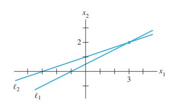
• 위 두개의 linear equation은 하나의 해만을 갖고 이를 그래프로 그리면 (3,2)한점에서 교차된다.

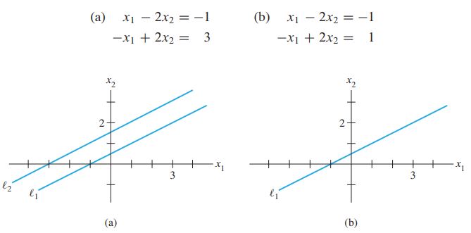
• (a)처럼 두 라인이 평행하여 해가 없는 경우도 있고, (b)처럼 두 라인이 모든 point에서 곂쳐 해가 무한대인 경우도 있다.

• 이러한 linear system을 일반화 시키면 다음과 같다.

A system of linear equations has

• 1. No solution
• 2. exactly one solution
• 3. infinitely many solutions

• 이때 2,3번인 단 하나의 해 혹은 무한개의 해를 가질 경우 linear system이 consistant 하다고 하고, 1번과 같이 해가 없을 경우 inconsistant 하다고 한다.

Matrix Notation

• 아래의 linear system을 두 형태의 Matrix form으로 나타내보자.

coefficient matrix
augmented matrix

Elemetary row operations

• Linear system은 augmented matrix form에서 아래 3개의 row operation을 사용하여 solution을 구하기 쉽게 변형시킬 수 있다.

Elemetary row operations

• 1. Replacement : 특정 row를 scaling시켜 다른 row에 더하여 소거.
  • $kR_i + R_j$
• 2. Interchange : 필요에의해 row를 바꿈.
  • $R_i \leftrightarrow R_j$
• 3. Scaling : nonzero constant k를 row에 곱해줌.
  • $kR_i$

• 이때 하나의 matrix를 sequence of row operation을 통해 transform시키면 두 matrix는 row equivalent 라고 한다.

• 또한 두 linear systme의 augmented matrix들이 row equivalent 하다면 두 system은 same solution set 을 갖는다.

1.2 Row Reduction and Echelon Forms

---

Echelon form

• 1. All nonzero rows are above any rows of all zeros.
  • 이때 nonzero row는 matrix의 특정 row의 element가 최소한 하나라도 0이 아닌 경우를 말한다.
• 2. Each leading entry of a row is in a column to the right of the leading entry of the row above it.
  • 특정 row의 leading entry의 위치가 자기잔보다 위에있는 leading enty보다 오른쪽에있다.
  • 이때 leading entry 는 모든 row의 "the leftmost nonzero entry" 를 뜻한다.

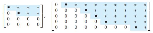
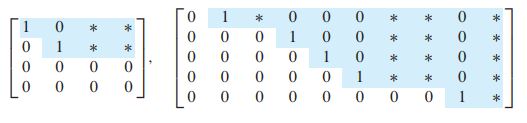
• 위와 같은 두 조건을 만족한 rectangular matrix를 echelon form이라고 하며 아래 그림과같은 형태가 된다.

Reduced echelon form

• 3. The leading entry in each nonzero row is 1.
• 4. Each leading 1 is the only nonzero entry in its column.

• Echelon form에서 추가로 위 두 조건을 만족한 rectangular matrix를 reduced echelon form이라고 하며 아래 그림과같은 형태가 된다.

Theroem 1
Uniqueness of the Reduced Echelon form

• Each matrix is row equivalent to one and only one reduced echelon matrix.
  • matrix를 row reduction해서 reduced echelon form으로 만들면 그 reduced echelon form은 unique하다.

Pivot Positions

• 직전에 언급하였듯이 특정 matrix의 reduced echelon form은 unique하기 때문에 해당 matrix의 어떤 echelon form이던 leading entry는 항상 같은 position을 갖는다.

A pivot position in a matrix A is a location in A that corresponds to a leading 1 in the reduced echelon form of A. A pivot column is a column of A that contains a pivot position.

The Row Reduction Algorithm

• 몇가지 step으로 이루어져 echelon form 혹은 reduced echelon form을 만드는 Row Reduction Algorithm을 살펴보자.

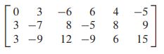
Step1
Begin with the leftmost nonzero column. This is a pivot column

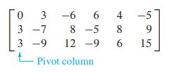
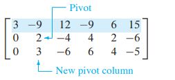
Step2
Select a nonzero entry in the pivot column as a pivot. If necessary, interchang rows to move this entry into the pivot position.

• Row1 과 row3를 interchange한다 (row2랑 바꿔도 노상관)

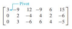
Step3
Row replacement operations to create zeros in all positions below the pivot.

• replacement operation을 사용하여 pivot position 아래의 모든 값들을 0으로 만들어준다. (add -1 times row 1 to row 2)

Step4
Cover (or ignore) the row containing the pivot position and cover all rows, if any, above it. Apply steps 1–3 to the submatrix that remains. Repeat the process until there are no more nonzero rows to modify.

• step3를 거쳐 pivot 아래의 값이 0으로된 row1 을 내두고 나머지 row들로 submatrix를 만들어 새로 pivot column과 pivot을 잡고 step1~3를 진행.

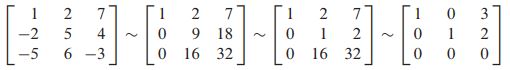
• 위 matrix처럼 step4까지 모두 마친 형태가 echelon form이 되는 것 이고 step1~4 까지의 과정을 row redunction algorithm의 "forward pahse라고 한다"

Step5
Beginning with the rightmost pivot and working upward and to the left, create zeros above each pivot. If a pivot is not 1, make it 1 by a scaling operation.

• Reduced echelon form을 만들어주기 위해 echelon form의 rightmost pivot부터 row operation을 통해 1로 만들고 pivot column의 나머지 요소를 0으로 만들어준다.

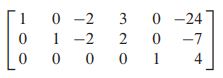
• 계산 과정은 생략하고 위 matrix가 최종 reduced echelon form으로 pivot column에 reading entry를 제외한 모든 element가 0이 된 것을 볼 수 있고 마지막 step5 과정을 "backward phase"라고 부른다.

Solutions of Linear Systems

• 이제 row reduction algorithm을 통해 linear system의 augmented matrix로 reduced echelon form을 만들 수 있게되었고 이를 통해 solutions을 구하는 것을 알아보자.

• 위 reduced echeoln form을 equation으로 나타내면 다음과 같다.
  
  

• 위 식을 전개한 general solution은 다음과같다.

• 각 reading position에 해당하는 $x_1, x_2$는 basic variable이라고 하고 $x_3$를 free variable이라고 한다.

• 이때 free variable인 $x_3$를 어떻게 선택하느냐에 따라 linear system의 sloution이 달라지는 형태이다 ("every solution of the system is determined by a choice of $x_3$")

Theorem 2
Existance and Uniqueness Theorem

• A linear system is consistent if and only if the rightmost column of the augmented matrix is not a pivot column—that is, if and only if an echelon form of the augmented matrix has no row of the form

• If a linear system is consistent, then the solution set contains either (i) a unique solution, when there are no free variables, or (ii) infinitely many solutions, when there is at least one free variable.

• free variable이 없으면 unique solution을 갖고 적어도 하나 있으면 infinitly many solution을 갖는다.

1.3 Vector Equations

---

Vectors in $\mathbb{R^n}$

Linear Combinations

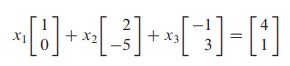
• vectors in $\mathbb{R^n}$ 이 $\bold{v_1, v_2, \cdots, v_p}$ 이고 scalars $\bold{c_1, c_2, \cdots, c_p}$가 주어졌을때 vector $\bold{y}$는 다음과같이 정의할수있다.

• 위와같은 형태를 "linear combination of $\bold{v_1, \cdots, v_p}$ with weights $\bold{c_1, \cdots, c_p}$" 라고 한다.

Example

• Let $\bold{a_1} = \begin{bmatrix} \;\;\;1\\-2\\-5 \end{bmatrix}$, $\bold{a_2} = \begin{bmatrix} 2\\5\\6 \end{bmatrix}$, $\bold{b} = \begin{bmatrix} \;\;\;7\\\;\;\;4\\-3 \end{bmatrix}$ . Determine whether $\bold{b}$ can be generated (or written) as a linear combination of $\bold{a_1}$ and $\bold{a_2}$.

• 위 linear combination을 활용하여 weighs $x_1, x_2$의 existance를 파악하고 solution을 구해보자.

• 일단 linear combination에 vector $\bold{a_1, a_2, b}$를 대입해보면 다음과같다.

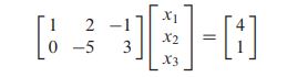
• 이를 linear system으로 나타내면 다음과 같고

• 이를 augmented matirx로 나타내어 row reduction하면 다음과 같다

• 위 예제를 통해 아래의 vector equation과 augmented matrix는 same solution set을 갖는다는 것을 알 수 있다.

Span

• Span{$\bold{v_1},\cdots,\bold{v_p}$} is the collection of all vectors that can be written in the form $c_1\bold{v_1} + c_2\bold{v_2} + \cdots c_p\bold{v_p} = \bold{b}$

• 즉 Span{$\bold{v_1},\cdots,\bold{v_p}$} 은 subset of $\mathbb{R^n}$ spanned by $\bold{v_1, \cdots, v_p}$ 이다.

• 또한 vector $\bold{b}$ is in Span{$\bold{v_1},\cdots,\bold{v_p}$} 은 위에서 보았던 linear combination과 augmented matrix이 solution을 갖는지 묻는 것과 동일하다.

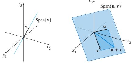
• Span{$\bold{v}$} 와 Span{$\bold{u,v}$}을 $\mathbb{R^3}$ space에서 나타내면 다음과같다.

1.4 The Matrix Equation Ax=b

---

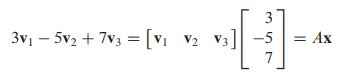
If A is an m x n matrix, with columns $\bold{a_1, \cdots, a_n}$ and if $\bold{x}$ is in $\mathbb{R^n}$, then the product of A and $\bold{x}$, denoted by A$\bold{x}$, is the linear combination of the columns of A using the corresponding entries in $\bold{x}$ as weights; that is,

• 이때 matrix A의 columns수는 vector $\bold{x}$의 enties수와 같다.

Matrix equation example

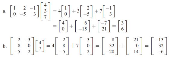
Vector equation to matrix equation example

Linear system to matrix equation example

• 위 세 예제 다 위에서 봤던 형태이다.

Existence of Solutions

Theorem 4
Let A be an m x n matrix. Then the following statements are logically equivalent.
a. For each $\bold{b}$ in $\mathbb{R^m}$, the equation A$\bold{x} = \bold{b}$ has a solution.
b. Each $\bold{b}$ in $\mathbb{R^m}$ ia a linear combination if the columns of A.
c. The columns of A span $\mathbb{R^m}$
d. A has a pivot position in every row. (A는 coefficient matrix임)

• Ax=b 형태의 matrix equation이 solution이 있다라는건 [A b] 형태의 augmented matrix가 echelon form으로 reduce했을때 [ 0 0 $\cdots$ 0 b ] 형태의 row가 나올수 없다는 것.

• 참고로 "Is Ax = b consistent?"와 "Is Ax = b consistent for all possible b?"는 조금 다른 문제이다 예제를 통해 살펴보자.

Example

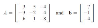
• Let A = $\begin{bmatrix} \quad 1 \quad 3 \quad 4 \\ -4 \quad 2 -6 \\ -3 -2 -7 \end{bmatrix}$ and $\bold{b} = \begin{bmatrix} b_1\\b_2\\b_3 \end{bmatrix}$. Is the equation A$\bold{x} = \bold{b}$ consistant for all possible $b_1,b_2,b_3$?

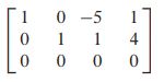
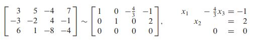
• matrix equation A$\bold{x} = \bold{b}$를 augmented form으로 row reduce시키면 다음과 같다.

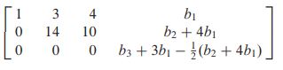
• Theorem2 에서 보았듯이 [0 0 0 b]와 같은 형태의 row에서 b가 nonzero이면 equation이 inconsistent하기 때문에 (for all possibel b가 아니라) 3번재 column의 b가 zero일때 equation이 consistent함을 만족한다.

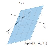
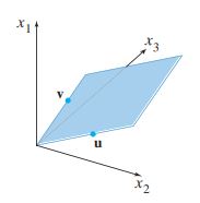
• 위 equation은 $\mathbb{R^3}$ space에서 원점을 지나는 평면이 되고 matrix의 column들의 linear combination으로 나타낼 수 있다.

Properties of the Matrix–Vector Product Ax

Theorem 5
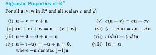
If A is an m # n matrix, u and v are vectors in Rn, and c is a scalar, then:

• a. A($\bold{u + v}$) = A$\bold{u}$ + A$\bold{v}$
• b. A(c$\bold{u}$) = c(A$\bold{u}$)

• 증명은 생략

1.5 Solution Sets of Linear System

---

Homogeneous Linear Systems

• Linear system을 위와같이 $m \times n$ matrix A와 $\mathbb{R^m}$ space의 zero vector로 표현된 식을 homogeneous equation이라고 한다.

• 이러한 system은 항상 $\bold{x}=0$인 적어도 하나의 solution을 갖게되고 이러한 solution을 trivial solution이라고 한다.

  • 이때 $\bold{x}=0$는 $\mathbb{R^n}$ space에서 모든 component가 zero인 vector를 말한다.

• $\bold{x}=0$가 아닌 non-zero vector인 $\bold{x}$은 "infinitely many solutios"을 갖게되며 이는 적어도 하나의 free variable을 갖는다는 뜻이다. 이를 nontrivial solution이라고 한다.

Example 1

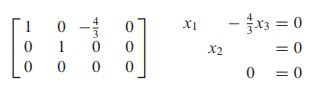
• Determine if the following homogeneous system has a nontrivial solution. Then describe the solution set.

• 위 system을 augmented matrix로 row reduction해서 reduced echelon form을 통해 general solution을 구하면 다음과 같고

• Free variable $\bold{x_3}$로 표현할 수 있는 general solution을 vector form으로 나타내면 다음과같다.

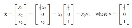
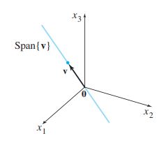
• 이때 solution set은 vector $\bold{v}$를 통해 나타낼 수 있고 이는 Span{$\bold{v}$} 를 뜻하고 아래 그림처럼 solution set이 line이 되는 것을 알 수 있다.

• 결과적으론 system이 nontrivial solution을 갖는다는 것을 알 수 있다.

Example2

• 이번엔 하나의 equation을 갖는 system의 homogeneous solution을 찾아보자.

• 위 식은 두개의 free variable로 표현 할 수 있으며 general solution을 vector로 나타내면 다음과같다.

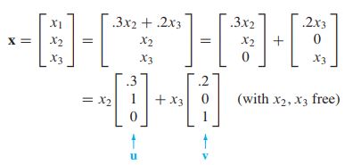
• 위와같이 두개의 free variable의 coefficient인 두 벡터를 통해 Span{$\bold{u,v}$} 로 solution set을 나타낼 수 있고 이는 아래의 그림처럼 평면이된다.

Parametric Vector Form

• 이러한 homogeneous의 solution set을 일반화 시키면 다음과 같이 나타낼 수 있고

• trivial solution은 $Span\{0\}$로 나타낼 수 있다.

• 그렇다면 위 example을 nonhomogeneous system에서 solution을 구하면 어떻게 나타날까?

Solutions of Nonhomogeneous Systems

Example3

• example1을 nonhomogeneous로 solution을 찾아보자.

• 이 전과 같이 위 식을 augmented form으로 row reduce하여 solution을 구하면 다음과같고

• 이를 vector로 나타내면 다음과 같다.

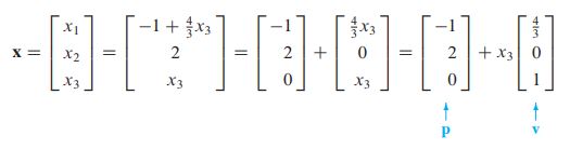
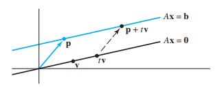
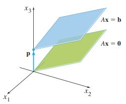
• 위 결과를 통해 nonhomogeneous의 solution과 homogeneous의 solution은 하나의 vector $\bold{p}$를 더해준 형태임을 볼 수 있고 이는 아래 그림처럼 nonhomogeneous의 solution이 homogeneous의 solution에 perallel한 solution sets임을 볼 수 있다.

Theorem 6

• Suppose the equation A$\bold{x}$ = $\bold{b}$ is consistent for some given $\bold{b}$, and let $\bold{p}$ be a solution. Then the solution set of A$\bold{x}$ = $\bold{b}$ is the set of all vectors of the form $\bold{w}$ = $\bold{p}$ + $\bold{v_h}$, where $\bold{v_h}$ is any solution of the homogeneous equation A$\bold{x}$ = $\bold{0}$.

• 결국 homogeneous의 solution $\bold{v_h}$를 알면 $\bold{p}$ + $\bold{v_h}$ 형태로 nonhomogeneous의 solution을 표현 할수 있고 이는 평행한 형태를 갖는다.

1.7 Linear Independence

---

Linearly independent

linearly independent

• An indexed set of vectors {$v_1, \cdots, v_p$} in $\mathbb{R^n}$ is said to be linearly independent if the vector equation $x_1\bold{v_1} + x_2\bold{v_2} + \cdots x_p\bold{v_p} = 0$ has only the trivial solution.

linearly dependent

• The set {$v_1, \cdots, v_p$} is said to be linearly dependent if there exist weights $c_1, \cdots, c_p$ , not all zero, such that $c_1\bold{v_1} + c_2\bold{v_2} + \cdots c_p\bold{v_p} = 0$
  • 이때 not all zero라는 것은 c (coefficient)가 적어도 하나만 nonzero이면 된다는 것.

• 위 처럼 homogeneous equation에서 trivial solution을 갖으면 vector set이 linearly independent 하고 nontrivial solution을 갖으면 linearly dependent 하다.

Example

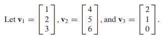
• 위 vector set이 linearly independent한지 dependent한지 살펴보자.

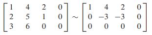
• 위 처럼 vector set을 homogeneous equation의 augmeted matrix을 row reduce하여 echelon form을보면 reduced echelon form을 구해서 general sloution을 구할필요도 없이 pivot을 보고 free variable 유무만 판단하여 non-trivial solution을 갖는다는 것을 알 수 있고 이를 통해 해당 vector set은 linearly dependent 하다는 것을 알 수 있다.

Sets of One Vector

• set이 $\bold{v}$ vector하나만을 갖고있고 $\bold{v}$가 non-zero vector라면 해당 set은 당연히 lineary independent하다.
  • $\because$ if $\bold{v} = 0$, $x_1\bold{v} = x_1 0 = 0$

Sets of Two Vectors

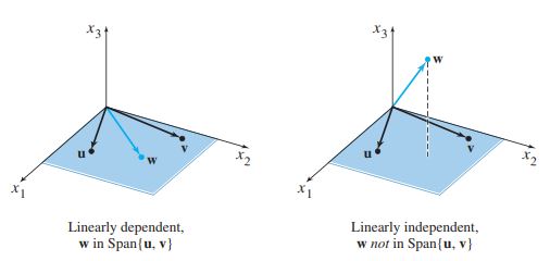
• A set of two vectors {$\bold{v_1, v_2}$} 가 linearly dependent 하다묜 한 vector는 다른 vector의 scalar multiplication이다.

Theorem 7
Characterization of Linearly Dependent Sets

• An indexed set $S = \{\bold{v_1}, \cdots, \bold{v_p}\}$ of two or more vectors is linearly dependent if and only if at least one of the vectors in S is a linear combination of the others.

• vector set이 2개이상 vector를 갖고 linearly dependent하다면 (non-trivial solution을 갖는다면) 적어도 하나의 vector는 나머지 vector의 linear combination으로 표현된다.

• 증명 생략

• A vector $\bold{w}$ is in $Span\{\bold{u, v}\}$ if and only if {$\bold{u, v, w}$} is linearly dependent (u, v중 적어도 하난 nonzero)

Theorem 8

• If a set contains more vectors than there are entries in each vector, then the set is linearly dependent. That is, any set $\{\bold{v_1}, \cdots, \bold{v_p}\}$ in $\mathbb{R^3}$ is linearly dependent if p > n

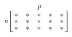
• 위 그림에서 pivot을 생각해보면 free variable이 무조건 있으므로 당연히 column vectos는 linearly dependent하다.

1.8 Introduction to Linear Transformations

---