이 글은 Linear Algebra and Its Applications 책을 정리한 글입니다.

2.1 Matrix Operations

---

Matrix의 표기법 및 용어

• m개의 rows와 n개의 columns를 갖은 $m\times n$ matrix의 $i$th row, $j$th column의 entry를 $a_{ij}$로 표기한다.

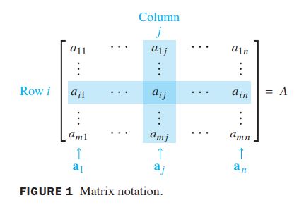
• 또한 $m\times n$ matrix A의 각 column을 vector in $\mathbb{R^m}$ 으로 다음과같이 표기할 수 있다

• $m\times n$ matrix의 $a_{11}, a_{22}, \cdots$ 를 diagonal entries 라고 하고 nondiagonal entries가 zero인 square $n\times n$ matrix를 diagoanl matrix 라고 한다

Theorem1
Let A,B and C be matrices of the same size, and let $r$ and $s$ be scalars
a. A + B = B + A
b. (A + B) + C = A + (B + C)
c. A + 0 = A
d. $r$(A + B) = $r$A + $r$B
e. ($r \ + \ s$)A = $r$A + $s$A
f. $r$($s$A) = ($rs$)A

• 위 theorem의 각 matrix를 column으로 쪼개서 봤을때도 ch1의 algebratic properties of $R^n$ (벡터의 성질)을 그대로 유지한다.

Matrix multipliaction

• $A(B\bold{x}) = (AB) \bold{x}$

• A를 $m\times n$ matrix, B를 $\bold{b_1}, \dots, \bold{b_p}$ 의 column vector를 가진 $n\times p$ matrix라고 하였을때 product AB 는 $m\times p$ matrix이며 $A\bold{b_1}, \dots, A\bold{b_p}$ 를 column 으로 갖는다

• matrix AB의 entry는 다음과같이 표현될 수 있다

Properties of Matrix Multiplication

Theorem2
Let A be an $m\times n$ matrix, and let B and C have sizes for which the indicated sums and products are defined.
a. A(BC) = (AB)C
b. A(B + C) = AB + AC
c. (B + C)A = BA + CA
d. $r$(AB) = ($r$A)B = A($r$B)
e. $I_m$A = A = A$I_n$

The Transpose of a Matrix

• Given an $m\times n$ matrix A, the transpose of A is the $n\times m$ matrix, denoted by $A^T$, whose columns are formed from the corresponding rows of A.

Theorem3
a. $(A^T)^T$ = A
b. $(A + B)^T = A^T + B^T$
c. For any scalar r, $(rA)^T = rA^T$
d. $(AB)^T = B^TA^T$

2.2 The Inverse of Matrix

---

Invertible Matrix

• n$\times$n matrix A가 invertible하다면 n$\times$n matrix C가 있을때 $CA = I$ and $AC = I$고 이때 $I$는 identity matrix이며 또한 matrix C는 invertible하며 unique하다.

• B를 또다른 A의 inverse라고 가정했을때 아래와 같이 결국 C는 unique하다

• matrix가 not invertible하다면 singular matrix, invertible하다면 nonsingular matrix 라고 한다.

Theorem4

Let A = $\begin{bmatrix} a \ b \\ c \ d \end{bmatrix}$. if ad-bc $\ne$ 0, then A is invertible and
$A^{-1} = \frac{1}{ad-bc}\begin{bmatrix}\quad d \ -b \\ -c \quad \ a \end{bmatrix}$.

if ad-bc = 0, then A is not invertible

• 이때 ad-bc를 determinent of A 라고 하며 det A 로 표기한다.

Theorem5

If A is an invertible n $\times$ n matrix, then for each $\bold{b}$ in $\mathbb{R}^n$,
the equation A$\bold{x} = \bold{b}$ has the unique solution $\bold{x} = A^{-1}\bold{b}$

Theorem6

a. If A is invertible matrix, then $A^{-1}$ is invertible and $(A^{-1})^{-1} = A$

b. If A and B are n$\times$n invertible matrices, then so is AB, and the inverse of AB is the product of the inverces of A and B in the reverse order.
That is $(AB)^{-1} = B^{-1}A^{-1}$

c. If A is an invertible matrix, then so is $A^T$, and the inverse of $A^T$ is the tranpose of $A^{-1}$. That is $(A^T)^{-1} = (A^{-1})^T$

Elemetary Matrices

• Elementary matrix란 1장에서 matrix를 echelon form으로 row reduction할때 쓰였던 single elementary row operation을 identity matrix에 수행한 것 이다. 다시말해 identity matrix 에 single elementary row operation 을 수행한 것 이고 다른 matrix에 Left multiplication(pre-multiplication)을 하면 single elementary row operation을 해준 것과 동일하다.

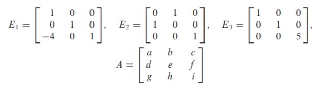
• 위 예시는 각각 replacement, interchange, scaling이며 임의 matrix A에 left multiplication을 해보면 다음과같다.

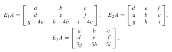
• 위와같은 elementary matrix $E$는 invertible하며 $E$의 inverse는 $E$가 identity matrix $I$에 row operation을 해주는 것이기에 다시 $I$로 다시 돌아가는 operation을 해주면 된다.
  
  

Theorme7
An n $\times$ n matrix A is invertible if and only if A is row equivalent to $I_n$, and in this case, any sequence of elementary row operations that reduces A to $I_n$ also transforms $I_n$ into $A^{-1}$

• 위에서 언급된데로 matrix A 가 invertible하다면 elementary matrix를 multiplication해주어 elementary row operation을 해주어 $I_n$을 만들고 elemetary matrix를 sequence로 나타내주면 inverse를 찾을 수 있다.
  
  
  $A \sim E_1A \sim E_2(E_1A) \sim \cdots ~ E_p(E_{p-1} \cdots E_1A) I_n \\ E_p \cdots E_1A = I_n \\ A^{-1} = (E_p \cdots E_1)^{-1}$

Algorithm for finding $A^{-1}$

• Row reduce the augmented matrix $[A \quad I ]$. If A is row equivalet to $I$, then $[A \quad I ]$ is row equinalent to $[I \quad A^{-1}]$. Otherwise, A does not have an inverse.

• 위 설명은 지금까지의 augmented matrix를 $[A \quad b]$ 로 표현하였는데 vector b대신 identity matrix I로 대신한 것이고 A부분이 I가되도록 계속 row reduction한 것이다.

Example

• Find the inverse of the matrix A, if it exists
  

Example

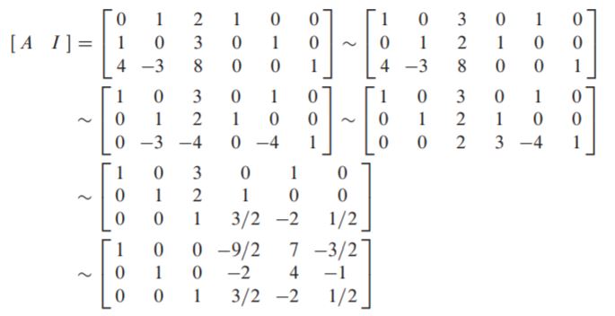
$[A \quad I ]$ 로 두었던 부분을 row reduction을 통해 I로 만들었으니 $I$자리의 matrix가 $A^{-1}$이 된다.

2.3 Characterizations of invertible matrices

---

Theorem8
Let A be a square n $\times$ n matrix. Then the following statements are equivalent.

• a. A is an invertible matrix.
• b. There is an n $\times$ n matrix C such that CA = I.
• c. The equation Ax = 0 has only the trivial solution.
• d. A has n pivot position.
• e. A is row equivalent to the idientity n $\times$ n matrix
• f. There is an n $\times$ n matrix D such that AD = I.
• g. The equation Ax = b has at least one solution for each b in $R^n$
• h. The columns of A span $R^n$.
• i. The linear transformation $\bold{x}\mapsto A\bold{x}$ maps $R^n$ onto $R^n$.
• j. The columns of A form a linearly independent set.
• k. The linear transformation $\bold{x}\mapsto A\bold{x}$ id one-to-one.
• l. $A^T$ is an invertible matrix.

• Invertible linear transformation
  - A linear transformation T : $R^n \to R^n$ is said to be invertible if ther exists a fuction S : $R^n \to R^n$ such that
  

2.4 Partitioned Matrices

---

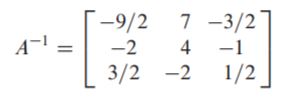
Theorem10
Column-Row Expansion of AB
If A is m $\times$ n and B is n $\times$ p, then

• 지금까지는 $[Ab_1 \quad \cdots Ab_n]$ 이런 식으로 A에 B의 column 벡터를 matrix multiplication한 것을 column으로두어서 나열한 표현을 썼었다.

2.5 Matrix Factorization

---

• Factorization이란 한 matrix를 두개 혹은 이상의 product로 다은과같이 표현하는 것이다.
  $A = BC$

LU Factorization

2.6 Subspace of $\mathbb{R^n}$

---

Definition
A subspace if $\mathbb{R^n}$ is any set $\bold{H}$ in $\mathbb{R^n}$ that has three properties :

• The zero vector is in $\bold{H}$
• For each $\bold{u}$ and $\bold{v}$ in $\bold{H}$, the sum $\bold{u} + \bold{v}$ is in $\bold{H}$.
• For each $\bold{u}$ and each scalar c, the vector $c\bold{u}$ is in $\bold{H}$.

• addition 과 scalar multiplication 에 닫혀있고, zero vector를 포함하고있으면 $\mathbb{R^n}$의 subspace가 된다.

Example

$\bold{v_1}$ and $\bold{v_2}$ and $\bold{H}$ = Span{$\bold{v_1}, \bold{v_2}$} 일때 $\bold{H}$가 $\mathbb{R^n}$의 subspace임을 보여라

라고 하였을때

위 식을통해 $\bold{u+v}$와 $c\bold{u}$ 는 $\bold{v_1}$과 $\bold{v_2}$의 linear combination으로 나타내어 addition 과 scalar multiplication 에 닫혀있음을 보일 수 있고음을 보일 수 있고 $0\bold{v_1} + 0\bold{v_2}$ 도 $\bold{v_1}$과 $\bold{v_1}$ 의 linear combination이므로 $\bold{H}$가 zero vector로 포함시켜 위 세가지 조건을 만족시키기에 $\bold{H}$는 $\mathbb{R^n}$의 subspace라고 할 수 있다.

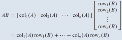
Example

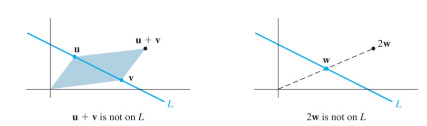
• 위 그림처럼 line $\bold{L}$이 원점(origin)을 지나지 않으면 addition 과 scalar multiplication 에 닫혀있지 않으므로 subspace가 될 수 없다.

$\therefore$ For $\bold{v_1}, \cdots, \bold{v_p}$ in $\mathbb{R^n}$, Span{$\bold{v_1}, \cdots, \bold{v_p}$} is a subspace of $\mathbb{R^n}$

Column Space and Null Space of a Matrix

Column space (Col A)

• The column space of a matrix A is the set Col A of all linear combinations of the columns of A.

  • $\mathbb{R^n}$ space의 column vector를 갖고있는 matrix A ( A = [$\bold{a_1}, \cdots, \bold{a_n}$] ) 일때 Col A 는 Span{$\bold{a_1}, \cdots, \bold{a_n}$}과 같은 표현이고 이 column space는 $\mathbb{R^n}$의 subspace이다.

Example

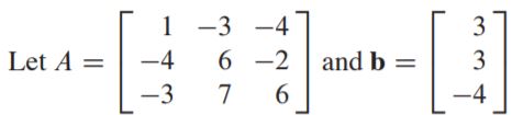
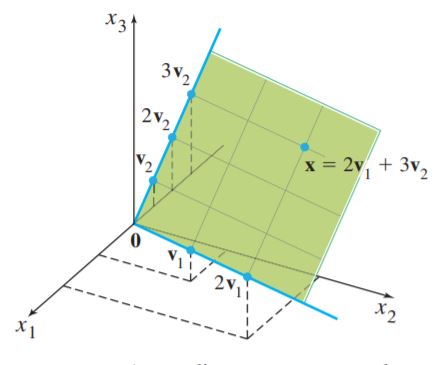
일 때, is $\bold{b}$ in Col A ?

• 위 matrix를 augmented matrix로 row reduce해주면 다음과 같고.

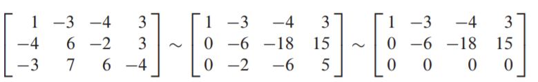
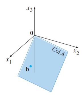
• 위 echelon form을 보면 pivot이 2개여서 A$\bold{x}$ = $\bold{b}$가 consistent함을 알 수 있고, 이는 vector $\bold{b}$ 가 matrix의 column vector들의 linear combination으로 나타낼 수 있음을 뜻하므로 $\bold{b}$ in Col A이다. 이를 그림으로 나타내면 다음과 같다.

Null space (Nul A)

• The null space of a matrix A is the set Nul A of all solutions of the homogeneous equation A$\bold{x}=0$

Theorem12
The null space of an m x n matrix A is a subspace of $\mathbb{R^n}$. Equivalently, the set of all solutions of a system A$\bold{x}=0$ of m homogeneous linear equations in n unknowns is a subspace of $\mathbb{R^n}$

• Nul A에 있는 어떤 $\bold{u, v}$ (homogeneous equation의 임의의 solution) 은 A$\bold{u} = \bold{0}$, A$\bold{v} = \bold{0}$ 두 식으로 나타낼 수 있고 이를 통해 A($\bold{u + v}$) = A$\bold{u}$ + A$\bold{v}$ = $\bold{0}$과 A(c$\bold{u}$) = A$\bold{u}$ + c(A$\bold{v}$) = c$\bold{0}$ = $\bold{0}$ 을 통해 addition과 scalar multiplication 에 닫혀 있음을 보임으로 Nul A 는 $\mathbb{R^n}$의 subspace임을 증명 할 수 있다.

Basis for a Subspace

• A basis for a subspace H of $\mathbb{R^n}$ is linearly independent set in H that spans H.

• Subspace는 무한대의 vector를 포함하고 있어 basis를 통해 최소한의 vector들로 subspace를 표현 할 수 있다.

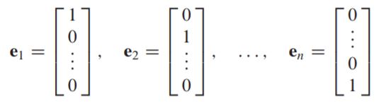
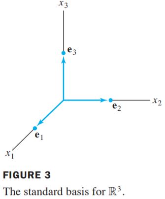
• 위와같은 identity matrix $I_n$의 column vector들은 linearly independent set 이며 $\mathbb{R^n}$의 standard basis 라고 한다.
  • 물론 $\mathbb{R^n}$도 $\mathbb{R^n}$의 subspace이다.

Example

• Nul A의 basis를 찾아보세요~

• 위 matrix의 homogeneous equation의 solution set은 null space이므로 augmented form으로 reduction해보면 다음과 같고,

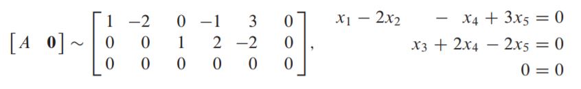
• 이를 free variable인 $x_2, x_4, x_5$를 통해 vector equation으로 general solution을 표현하면 다음과 같다.

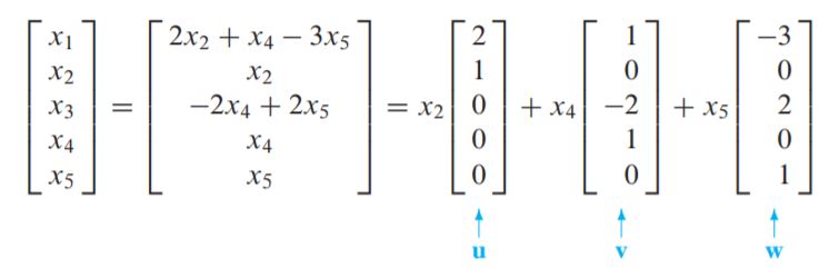
• vector $\bold{u, v, w}$으로 나타낼 수 있는 linear combination은 Nul A 가 되고 위 linear combination은 자동적으로 trivial solution을 갖기에 (vector $\bold{X}$를 0으로 만드는 free variable $x_2, x_4, x_5$는 모두 0이 됨) vector $\bold{u, v, w}$는 linearly independent set이고 {$\bold{u, v, w}$} 는 Nul A 의 basis 가 된다.

Example

• 이번엔 Col B의 basis를 찾아보세요~

• 위 reduced matrix B의 column들을 $b_1, \cdots, b_5$ 라고 하였을 때 당연하게도 아래 식처럼 다른 column들은 pivot column인 $b_1, b_2, b_5$의 inear combination으로 표현 할 수 있고

• pivot column인 $b_1, b_2, b_5$는 당연히 linearly independent set이므로 {$b_1, b_2, b_5$} 는 Col B 를 span한다.

• $\therefore$ pivot columns of B {$b_1, b_2, b_5$}는 Col B의 basis이다.

• 위 matrix A을 row reduction하면 matirx B가 되지만 Col A $\neq$ Col B이다.

  • row operation 이라는게 column이 아니라 row간 계산을 수행하므로 pivot column을 바꿀 수 없고 결과적으로 column간 linear dependence 관계에 영향을 미치지는 못한다.

  • 결론은 row equivalent한 matrix들은 pivot column들이 동일하여 해당 matrix의 동일 위치의 pivot column들이 column space에 basis가 되긴 하지만 column space들은 동일 공간에 있다고 볼 수 없다.

Theorem13
The pivot columns of a matrix A form a basis for the column space of A.

2.7 Dimension and Rank

---

Coordinate Systems

Definition
Suppose the set $\mathcal{B}$ = {$\bold{b_1}, \cdots, \bold{b_p}$} is a basis for a subspace H. For each $\bold{x}$ in H the coordinates of x relative to the basis $\mathcal{B}$ are the weights $\bold{c_1}, \cdots, \bold{c_p}$ such that $\bold{x} = c_1\bold{b_1}+ \cdots + c_p\bold{b_p}$, and the vector in $\mathbb{R^p}$

is called the coordinate vector of x (relative to $\mathcal{B}$) or the $\mathcal{B}$-coordinate vector of x

• basis $\mathcal{B}$ 라는 것은 일반적인 좌표계가 아닌 basis에 대한 좌표계를 나타내며 위 definition은 basis가 주어졌을 때 H의 특정 vector $\bold{x}$를 나타내는 weights(coefficient) $\bold{c_1}, \cdots, \bold{c_p}$는 unique하다는 것을 나타낸다.

Example

• vector $\bold{x}$가 subspace H = Span{$\bold{v_1, v_2}$}에 있는지 보이고 $\mathcal{B}$-coordinate vector of $\bold{x}$를 구해라

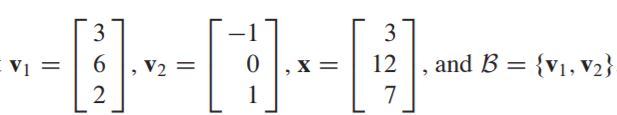
• 일단 $\bold{v_1, v_2}$는 서로 scalar 곱으로 표현될 수 없어서 linearly independent하고 subspace H의 basis가 될 수 있다.

• 위 vector들을 augmented matirx로 reduction하면 다음과 같고

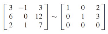
• vector equation $c_1\bold{v_1} + c_2\bold{v_2} = \bold{x}$ 일 때 $c_1 = 2, c_2 = 3$ 이므로 $\left [ \bold{x} \right ]_\mathcal{B} = \begin{bmatrix} 2 \\ 3 \end{bmatrix}$이 되며 basis $\mathcal{B}$는 subspace H의 "coordinate system"이 된다. 그림으로 나타내면 다음과 같다.

• 위 그림에서 보다시피 basis의 vector들($\bold{x_1, x_2}$)은 $\mathbb{R^3}$에 있지만 subspace H에있는 $\bold{x}$들은 cordinate vector에 의해 마치 $\mathbb{R^2}$에 있는것 처럼 동작한다 이를 H is isomorphic to $\mathbb{R^2}$ 이라고 부른다.

The Dimension of a Subspace

Definition
The dimension of a nonzero subspace H, denoted by dim H, is the number of vectors in any basis for H. The dimension of the zero subspace {$\bold{0}$} is defined to be zero.

• nonzero subspace H의 basis는 여러개일 수 있지만 dimension은 똑같다는 소리.

• $\mathbb{R^n}$ space는 n dimension을 갖고 모든 $\mathbb{R^n}$의 모든 basis는 n개의 vector를 갖는다.

  • 이때 0을 지나는 subspace가 평면이면 two-dimensional이고, line이면 one-dimensional이다.

Rank

definition
The rank of a matrix A, denoted by rank A, is the dimension of the column space of A.

Example

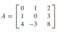
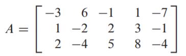
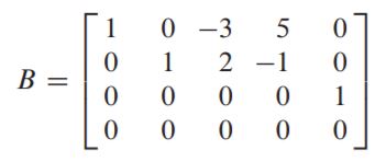
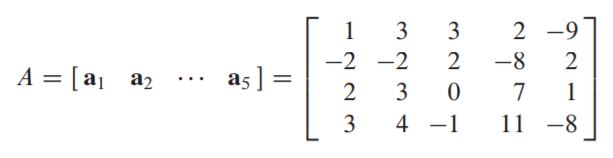
• 아래 matrix A의 rank는????

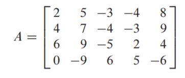
• 우선 rank A는 Col A의 basis의 dimension을 말하므로 matrix의 echelon form을 구하면

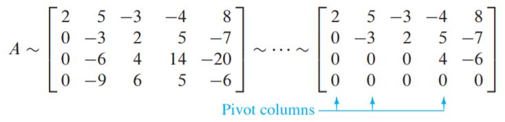
• row reduction한 echelon form은 3개의 pivot column이 있는걸 알 수 있고 이는 원래의 matrix A의 pivot column과 위치가 같으므로 rank A = 3 임을 알 수 있다.

• 이때 A$\bold{x}$ = $\bold{0}$은 두개의 free variable을 갖는데 이는 5개 column중 2개의 non-pivot column이 있다는 것을 통해 바로 알 수 있고 $x_3\bold{u} + x_5\bold{x}$ 로 general solution의 vector equation을 나타낼 수 있는데 이를 통해 null space A의 dimension (dim Nul A)는 free variable의 개수와 같은 것을 알 수 있다.

<Theorem 14> The Rank Theorem
if a matrix A has n columns, then rank A C dim Nul A D n

<Theorem 15> The Basis Theorem
Let H be a $\mathcal{p}$-dimensional subspace of $\mathbb{R^n}$. Any linearly independent set of exactly $\mathcal{p}$ elements in H is automatically a basis for H. Also, any set of $\mathcal{p}$ elements of H that spans H is automatically a basis for H.

The Invertible Matrix Theorem (cont'd)

• m. The columns of A form a basis of $\mathbb{R^n}$.
• n. Col A = $\mathbb{R^n}$
• o. dim Col A = n
• p. rank A = n
• q. Nul A = {$\bold{0}$} : null space가 zero vector밖에 없고 trivial solution을 갖는다는 소리.
• r. dim Nul A = 0