이 글은 Linear Algebra and Its Applications 책을 정리한 글입니다.

3.1 Introduction to Determinants

---

• 2장에서 2 $\times$ 2 matrix A = $\begin{bmatrix} a \ b \\ c \ d \end{bmatrix}$가 있을때 det A = ad-cd 라는것을 보았었고 만약 A가 invertible하다면 det A 는 nonzero 여야한다는 것을 보았다.

• 이러한 사실을 토대로 3 $\times$ 3 matrix의 determinant를 살펴보며 matrix의 determinant의 definition을 알아본다.

• 위 3 $\times$ 3 matrix를 row reduction 해보면 다음과같다.

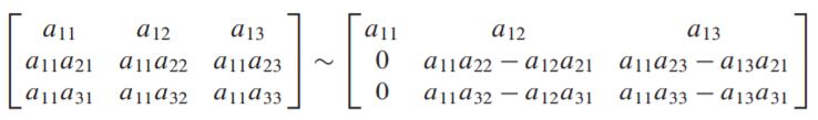
• 이때 matrix A가 invertible하다고 가정했을때 (2,2)-entry 또는 (3,2)-entry는 nonzero가 된다 (2장에서 보았듯이 n$\times$n matrix가 invertible하다면 n개의 pivot이 있어야함). 이를 또 전개하면 다음과같다.

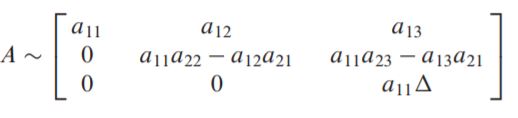
• 이때 $\Delta$ = $a_{11}a_{22}a_{33} + a_{12}a_{23}a_{31} + a_{13}a_{21}a_{32} - a_{11}a_{23}a_{32} - a_{12}a_{21}a_{33} - a_{13}a_{22}a_{31}$ 가 된다.

• A가 invertible이라고 가정하였기 때문에 $\Delta$도 nonzero가 되어야 하며 $\Delta$를 우리가 봤던 2x2 matrix의 determinants로 정리하면 다음과 같다.

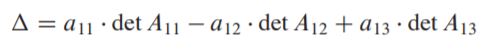
• 이때 $A_{ij}$ 로 표기된행렬은 원래의 matrix A에서 i-th row와 j-th column을 제외한 나머지를 뜻한다.

Definition


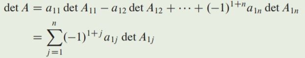
For n $\ge$ 2, the determinant of an n $\times$ n matrix A = [$a_{ij}$] is the sum of n terms of the form $\plusmn a_{1j}detA_{1j}$, with plus and minus signs alternating, where the entries $a_{11} \ \cdots \ a_{nn}$ are from the first row of A.

• 

• 이때 A가 5x5 라고 했으면 det$A_{1n}$의 형태는 4x4 형태이니 또 해당 matrix의 determinant는 3x3 matrix고 점점 줄어드는 형태로 표현 가능하다.

Example

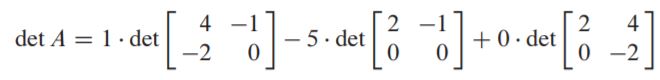
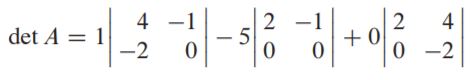
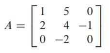
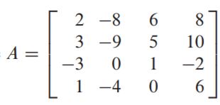
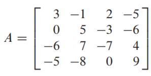
• 아래 matrix A의 determinant를 구해보자.

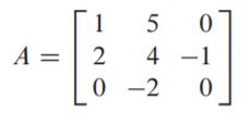
• 위에서 보았던 3x3의 determinant는 $a_{11}detA_{11} - a_{12}detA_{12} + a_{13}detA_{13}$ 이며 이것은 아래돠같이 matrix로 표현된다.

Cofactor

• Determinant는 다음과 같이도 나타낼 수 있다.

• 이를 좀더 편리하게 표현하기 위해 또 다른 표현법이 있다.

• Given A =[$a_{ij}$], the (i,j)-cofactor of A is the number $C_{ij}$ given by $C_{ij} = (-1)^{i+j} \sdot detA_{ij}$

• 이러한 fomula를 a cofactor expansion across the first row of A 라고 한다.

Theorem1


The determinant of an nxn matrix can be computed by a cofactor expansion across any row or down any column. The expansion across the i-th row using the cofactor is
$detA = a_{i1}C_{i1} + \cdots + a_{in}C_{in}$
The cofactor expansion down the j-th column is
$detA = a_{1j}C_{1j} + \cdots + a_{nj}C_{nj}$

• cofactor expansion $C_{ij}$의 plus or minus sign 은 다음과같다.

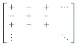
• 위 이론에 대한 증명은 pass하지만 언급된 것 처럼 determinant를 cofactor expansion으로 표현할 때 i-th row로 표현할 수도 있고, j-th column으로 표현할 수도 있다.

• 또한 이전에 보았던 3x3 matrix의 determinant인 $\Delta$ = $a_{11}a_{22}a_{33} + a_{12}a_{23}a_{31} + a_{13}a_{21}a_{32} - a_{11}a_{23}a_{32} - a_{12}a_{21}a_{33} - a_{13}a_{22}a_{31}$ 에서 얘들을 어떻게 묶느냐에 따라 determinant cofactor expansion이 i-th row인지 j-th column인지 표현할 수 있는 것 이다.

Example

• 아래 matrix를 cofactor expansion을 통해 나타내고 determinant를 구해보자.

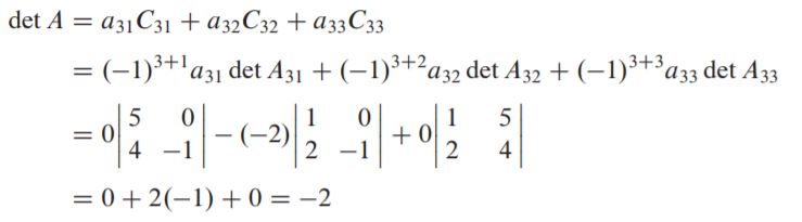
• 위 solution처럼 0이 많이 끼어있는 row or column을 골라 쉽게 계산 할 수 있다.

Theorem2


if A is a triangular matrix, then det A is product of the entries on the main diagonal of A.

Example

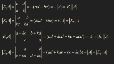
• 아래와같이 matrix A와 elementary matrix e1_e4 가 주어졌을때 Verify detEA = (detE)(detA)

$E_1 = \begin{bmatrix} \ 0 \ 1 \ \\ \ 1 \ 0 \ \end{bmatrix} , \quad E2 = \begin{bmatrix} \ 1 \ 0 \ \\ \ 0 \ k \ \end{bmatrix} , \quad E3 = \begin{bmatrix} \ 1 \ k \ \\ \ 0 \ 1 \ \end{bmatrix} , \quad E4 = \begin{bmatrix} \ 1 \ 0 \ \\ \ k \ 1 \ \end{bmatrix}$

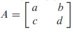
• |$E_1$| = -1, |$E_2$| = k, |$E_3$| = 1, |$E_4$| = 1, |$A$| = ad-bc이다 외워두면 좋다.

3.2 Properties of Determinant>

---

• 이번 챕터에서는 matrix에 row operation을 행할 때 어떻게 변하는지 알아보려한다.

Theorem3

• Let A be a square matrix
  a. If a multiple of one row of A is added to another row to produce a matrix B, then det B = det A (row operation할 경우)
  b. If two rows of A are interchanged to produce B, then det B = -detA
  c. If one row of A is multiplied by k to produce B, then det B = k$\sdot$detA

• 직전의 example에서 보았듯이 detEA = (detE)(detA) , det E = 1, -1 or r .

• 전장에서 보았듯이 n = 2일때는 참이고 when n = 3 일때는 B = EA이고 E에 영향을 받지 않는 row를 i라고 하였을 때 $detB_{ij} = \alpha \sdot detA_{ij}$이다 (이는 2x2 matrix에서 봄) cofactor expansion을 통해 나타내면,

Example

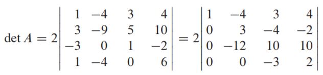
• 아래 matrix A 에서 det A를 구해보자.

• 위 matrix를 row operation을 취해 upper triangular matrix로 나타내면 다음과같다.

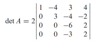
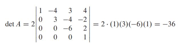
• theorem2에서 언급한데로 upper triangular matrix의 determinant는 product of the entries on the main diagonal of A 기에 위와같이 곱해주어 구한다.

• 만약 pivot을 포함하지 않은 row가 있었으면 이전 장에서 언급된 것 처럼 singular matrix(not invertible) 이고 A의 triangular 형태에서 diagonal term들 중 하나는 0 이므로 A의 determinant는 0이된다.

• invertible 하다면 reduced echelon form은 unique하지만 그냥 U(echelon form)은 pivot들의 값이 다르게 여러형태가 나올 수 있지만 그것들의 곱인 determinant는 결국 같다. 각 pivot들은 det 형태로 밀접한 관계가 있다는 소리.

Theorem4

• A square matrix A is invertible if and only if det A $\ne$ 0

• det A = 0 이면 row나 column들이 linealy dependent 하다는 것이니 non trivial solution을 갖는다

Example

• 아래 matrix A 에서 det A를 구해보자.

solution

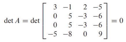
• row operation을 하다보면 row2와 row3이 같아지기에 detA = 0
  -> row2와 row3이 같다는것은 pivot이 n개가 아니란 것이고 이는 not invertible이며 free variable을 갖고 homogeneous equation에서 non-trivial solution을 갖는다는 것이다.

Theorem5

• If A is an nxn matrix, then $detA^T = detA$

증명 생략

Theorem6 Multiplicatative Property

• If A and B are nxn matrix, then detAB = (detA)(detB)

증명 생략

• detA+B $\ne$ detA + detB in general.

Example

• 아래 matrix A, B를 통해 위 Themorem6를 증명해보여라.

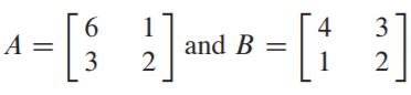
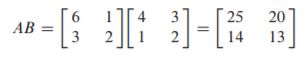
• 계산해 보면 det AB = 45 이지만 det A = 9 , det B = 5 이기에 detA+B $\ne$ det A + det B 이다.

3.3 Cramer's rule, volumne and linear transformation

---

• 이번 섹션은 이전 섹션의 이론들을 적용시켜보고 determinant의 geometric 해석을 살펴본다.

Cramer's rule

• cramer's rule은 3x3 이상의 matrix에서 A$\bold{x} = \bold{b}$와 같은 equation의 해카 b의 entries가 변할때 어떻게 바뀌는지 와같은 복잡한 계산식에서의 편의를 위해 사용된다.

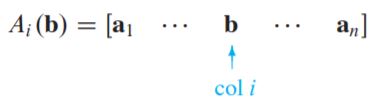
• n$\times$n matrix A와 any b in $R^n$이 있을때, $A_i(b)$ 는 아래와 같이 A의 i-th column vector를 $\bold{b}$로 치환한 것이다.

Theorem7 Cramer's rule

• Let A be an invertible n$\times$n matrix. For any b in $R^n$, the unique solution x of Ax = b has entries given by
  $x_i = \frac{detA_i(b)}{detA}, \quad i = 1,2 \cdots, n$

• 위 이론은 solution x를 표현하는 방법이다.

• nxn matrix A와 identity matrix I의 column들을 통해 나타내보면 다음과같다.

• $A \sdot I_i(x)$ 와 $A_i(b)$에 각 det를 취하면 다음과같다.

Example

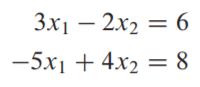
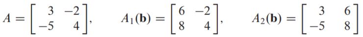
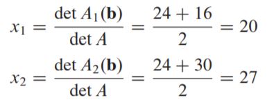
• Cramer's rule을 통해 아래 system의 solution을 구해보자.

A Fomula for $A^{-1}$

• Cramer’s rule 은 n$\times$n matrix A의 inverse를 명시적으로 쉽게 나타낼 수 있다.

• A$\bold{x} = e_j$ 의 식이 있을 때 solution은 $\bold{x}=A^{-1}e_j$ 과같이 나타낼 수 있으며
  (i-j) entry of $A^{-1}$은 cramer's rule을 통해 $x_i = \frac{det A_i(e_j)}{det A}$로 나타낼 수 있다.
  

• 원래의 $\bold{b}$를 $e_j$로 두었기 때문에 $A^{-1}$의 i-th row, j-th column인 entry가 되는 것.

• i-th column을 치환하여 cramer's rule로 나타낸 것 이고, inverse의 성질을 보았을때 $\bold{x} = A^{-1}e_j$ 즉 solution vector x의 j-th row이다.

이때 i와 j, row와 column을 matrix A의 입장에서 나타낸 것이라 inverse의 entry로 나타낼때 거꾸로가 되는데 졸라 햇갈린다~.

• 그렇기에 $detA_i(e_j)$ 을 j-th column으로 cofactor expansion하면 $C_{ji} = (-1)^{j+i} \sdot detA_{ji}$ 이며 전개하여 나타내면 아래와같다.

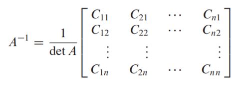
• 이때 위 matrix 형태를 adjugate of A 혹은 adj A 라고 한다.

Theorme8

• Let A be an invertible n $\times$ n matrix, then $A^{-1} = \frac{1}{detA}\ adjA$

Example

• Matrix A의 inverse를 구하시오.

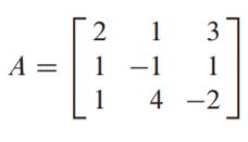
• adj A 를 구하기위해 cofactor들을 계산하면 다음과 같고

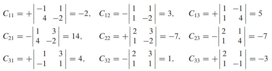
• determinant를 따로 계산하면 다음과같이나온다.

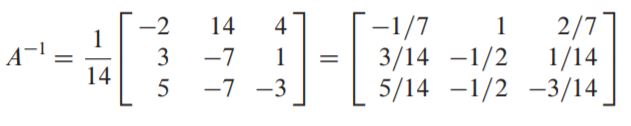
• 이처럼 사실 $A^{-1}$를 구할때는 row reduction 하는 것 보다 훨씬 복잡하고 비효율적이지만 cramer's rule을 통해 다른 이론을 유도할때 유용하게 쓰인다.

Determinant as Area or volume

• Determinant는 area와 volume에 매우 밀접한 관계를 갖는데 geometric 해석을 통해 이를 살펴보자.

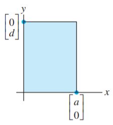
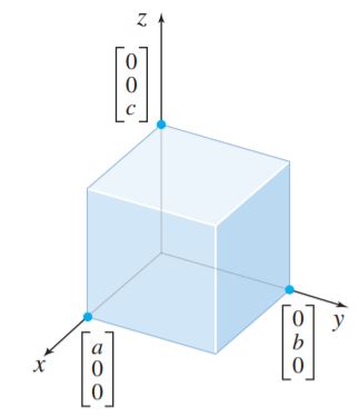
Theorem9

• If A is a 2x2 matrix, the area of the parallelogram(평행사변형) determined by the columns of A is |det A|
• The volumn of parallelepiped(평행육면체) determined by the columns of A is |det A|

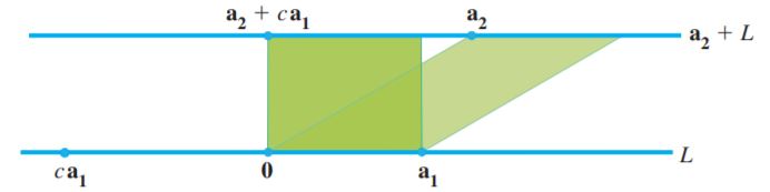
• 두 사각형의 면적은 determinant로 구할 수 있고 위처럼 matrix 형태에서 row replacement 한 형태의 area를 구해여도 같다.

• 이는 이전에 배운 것 처럼 (detE)(detA) = detEA 에서 살펴볼 수 있다.

이후 내용은 그림그리기 어려우니 pass

Linear Transformation