Intro...

---

• 이번에 리뷰할 Identity Mappings in Deep Residual Networks는 지난 ResNet논문의 연구팀이 Identity mapping에 대한 고찰을 통해 ResNet의 성능이 왜 좋은지 검증하였고 여러 시도를 통해 개선된 architecture를 선보인 논문이다.

Analysis of Deep Residual Networks

---

• 이전 논문에서 소개된 original residual unit은 다음과같은 식을통해 나타낼 수 있다.
  
  

  $\bold y_l = h(\bold x_l) + \mathcal F(\bold x_l, W_l), ~~~~~ (1)\\ \bold x_{l+1} = f(\bold y_l) ~~~~~ (2)$
  
  

• 위 식의 변수들과 첨자는 다음과같다.

  • $\bold x_l$ : l-th Residual unit의 input feature
  • $W_l = \{ W_{l,k} |_{1 \le k \le K} \}$ : l-th Residual unit의 weights (K is 2 or 3)
  • $\mathcal F$ : Residual function (e.g. a stack of two 3x3 conv layers )
  • $f$ : ReLU
  • $h$ : identity (shortcut) mapping

• 이때 $f$가 identity인 경우 ($\bold x_{l+1} \equiv \bold y_l$)인 경우 첫번째 식과 두번째 식을 합쳐볼 수 있다.
  
  

  $\bold x_{l+1} = \bold x_l + \mathcal F(\bold x_l, W_l) ~~~~~ (3)$
  
  

• $(\bold x_{l+2} = \bold x_{l+1} + \mathcal F(\bold x_{l+1}, W_{l+1}) ) = \bold x_l + \mathcal F(\bold x_l, W_l) + \mathcal F(\bold x_{l+1}, W_{l+1})$ 위와같이 Eqn.(3)를 Recursive하게 계속 대입하면 다음과 같이 표현할 수 있다.
  
  

  $\bold x_L = \bold x_l + \sum_{i=1}^{L-1} \mathcal F(\bold x_i, W_i) ~~~~~ (4)$
  
  

• 위 Eqn.(4)는 다음과같은 두가지 특성을 보여준다.

  (i) deeper unit $L$의 feature $\bold x_L$ 은 shallowe unit $l$의 feature $\bold x_l$ 과 $\sum_{i=1}^{L-1} \mathcal F$ 형태의 residual function의 합으로 표현할 수 있으며 이는 model이 unit $L$ 과 unit $l$ 사이에서 residual fashion으로 존재한다는 것을 나타낸다.

  (ii) 어떠한 deep unit $L$에 대하여 feature $\bold x_L = \bold x_0 + \sum_{i=1}^{L-1} \mathcal F(\bold x_i, W_i)$ 은 이전의 모든 residual functions의 outputs의 $summation$으로 표현되며 (+ $\bold x_0$), 이와 반대로 "plain network"에서의 feature $\bold x_L$은 $\prod_{i=0}^{L-1} W_i \bold x_0$ 형태의 a series of matrix-vector products 즉, matrix vector poroduct의 거듭연산 형태로 나타난다.

• Eqn.(4)는 backward propagation에서도 중요한 특성을 갖도록 유도한다.

• $\varepsilon$을 loss function이라고 했을때 back-prop에서의 chain rule을 통해 다음과 같은 식을 가질 수 있다.
  
  

  $\frac{\partial \varepsilon}{\partial \bold x_l} = \frac{\partial \varepsilon}{\partial \bold x_L} \frac{\partial \bold x_L}{\partial \bold x_l} = \frac{\partial \varepsilon}{\partial \bold x_L} \biggl(1 + \frac{\partial}{\partial \bold x_L} \sum_{i=1}^{L-1}\mathcal F(\bold x_i, W_i) \biggr) ~~~~~ (5)$
  
  

• Eqn.(5)는 gradinet $\frac{\partial \varepsilon}{\partial \bold x_l}$ 을 두개의 additive term으로 decompose하여 해석해 볼 수 있다.

  • $\frac{\partial \varepsilon}{\partial \bold x_L}$ term은 어떠한 weights layer도 거치지 않고 directly하게 propagates된다는 것을 보장하고.

  • $\frac{\partial \varepsilon}{\partial \bold x_L}(\frac{\partial}{\partial \bold x_L} \sum_{i=1}^{L-1}\mathcal F )$ term은 propagate때 weights layer를 거치지만 일반적으로 mini-batch의 모든 sample마다 $\frac{\partial}{\partial \bold x_L} \sum_{i=1}^{L-1}\mathcal F$ 가 항상 -1이 되어 전체 식이 0이 될 가능성은 극히드물기에 gradinet $\frac{\partial \varepsilon}{\partial \bold x_l}$ 이 "canceled out"될 경우는 없다고 봐도 무방하다. 즉, gradient vanishing이 발생할 가능성은 없다는 것이다.

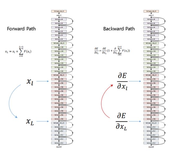
• 정리하면 Eqn.(4)를 통해 forward-pass시 residual unit의 identity mapping(shortcut connection)을 이용해 곱셈의 누산이 아닌 덧셈으로 쉬운 정보이동(directly propagated information)이 가능해지며, Eqn.(5)를 통해 수많은 layer의 weights matrix들이 곱셈을 통해 backprop되는게 아니기에 gradient vanishing문제가 발생하지 않는다는 것이다.

• 이를 그림으로 한눈에 표현하면 다음과 같다.

Improving Architecture

---

• 논문에선 Residual unit의 구조를 Identity mapping이 적용되는 두가지 요소 Skip Connections(Shortcut) 과 Activation Fcuntion으로 나누어 실험을 진행하였다.

Skip Connections

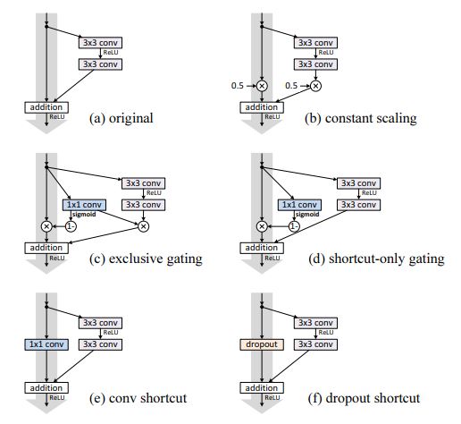
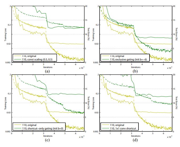
• 논문에서는 original architecture (a)와 더불어 shortcut에 다양한 variation을 주어 110-layer의 ResNet에 CIFAR-10을 사용하여 실험을 진행하였다.

• 위 그림처럼 실험 결과는 oritinal architecture의 error rate가 가장 낮았다.

• 이를통해 (b)~(f) 구조는 shortcut에 multiplication형태가 추가되면 정보가 directly하게 전달되지 못하고 blocking되어 최적화에 문제가
  생길수 있으므고 결과적으로 identity skip connection이 최적화를 쉽게한다고 볼 수 있다.
  
  

* 각 archetecture에대한 자세한 설명은 해당 논문에 자세히 설명되어 있다.

Activation Fcuntion

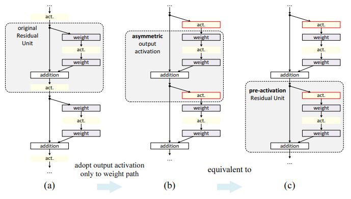
• 논문 저자들은 activation function(ReLU)의 위치가 어떤 영향을 주는지 확인하기 위해 아래와같이 다양한 variation을 주어 실험하였다.

• orininal의 구조를 보면 activation이 shortcut과 BN모두에 영향을 끼치는 형태이다. 이는 Eqn.(1), Eqn.(2)를 통해 $\bold y_{l+1} = f(\bold y_l) + \mathcal F(f(\bold y_l), W_{l})$ 로 나타낼 수 있었다.

• 이 구조를 조금 변형하여 $\mathcal F$에만 activation을 적용하여 $\hat f$으로 나타내어 $\bold y_l = f(\bold y_l) + \mathcal F(\hat f(\bold y_l), W_l)$으로 표현할 수 있고 $\bold y_l$만 $\bold x_l$로 바꿔주어 다음과같은 식으로 나타낼 수 있다.

• 이는 Eqa.(3)와같은 형태를 을 만족하기위해 ($\bold x_{l+1} \equiv \bold y_l$) 라는 가정을 통해 Eqa.(1), Eqa.(2)에서 f를 identity mapping인 것 처럼 만들기 위함이다.
  - 실제로 ReLU자체를 identity하게 만든게 아니라 x 자체를 identity하게 만들어주기 위함이다(말이 어렵지만 앞선 식의 가정을 설명하기위함이다...)

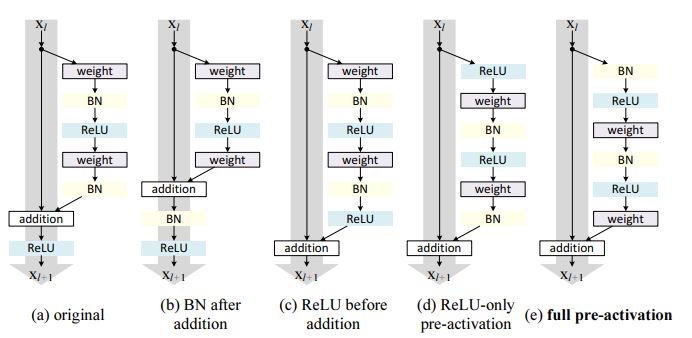
• 이를 그림으로 나타내면 다음과 같다.

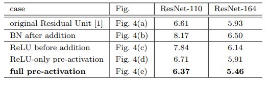
• 위 그림처럼 activation의 위차가 weights layer앞쪽으로 오면서 pre-activation 구조가 되며 이러한 구조에서 BN을 ReLU앞으로 옮겨 (e) 구조의 "full-pre activation" 형태가 된다.

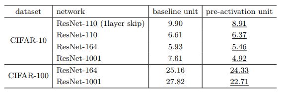
• 이러한 "full-pre activation" 구조를 사용한 실험 결과는 다음과 같으며.

• 이때 특이한 결과를 확인할 수 있다.

• 위 그림을 보면 Pre-activation을 적용한 경우 test error가 original에 비해 낮아진 것을 볼 수 있지만, traning에서는 iteration이 커질 수록 original보다 결과가 안좋다는 것을 볼 수 있다.

• 논문에서는 이러한 결과가 test set에선 pre-activation을 사용하여 최적화가 쉬워져 성능이 좋아졌고, training시엔 BN이 regularization역할을 수행하여 generalization이 잘 되어 over-fitting을 줄였다고 설명하고있다.

Outro...

---

• 이 논문에서는 identity mapping에 대한 고찰을 통해 residual block의 구조를 shortcut과 activation function 관점에서 여러 실험을 하였고 결론적으로 original shortcut구조에 pre-activation을 사용하여 성능을 향상시켰다.

• 개인적으로 이 전 논문과 함께 해당 논문이 왜 이러한 구조가 성능을 향상시키는지에 대한 고찰을 잘 설명하고있어 좋은 인사이트를 얻었다. Kaiming He의 He initialization을 설명한 논문에서도 느꼈지만 그냥 이사람이 설명을 잘하는건가 싶다.

References

• Identity Mappings in Deep Residual Networks

• EECS 498-007 / 598-005 Deep Learning for Computer Vision

• 라온피플