Introduction

• In 1960, Rudolf Kalman developed a way to solve some of the practical difficulties that arise when trying to apply Weiner filters
• The three keys to leading to the Kalman filter
  • Wiener filter : LMMSE of a signal (only for stationary scalar signals and noises)
  • Sequential LMMSE : sequentially estimate a fixed parameter
  • State-space models : dynamical models for varying parameters
• Kalman Filter : sequential LMMSE estimation for a time-varying parameter vector, but the time variation is constrained to follow a state-space dynamical model(allow the unknown parameters to evolve in time)
• Kalman filter is an optimal MMSE estimator for jointly Gaussian case, and is the optimal LMMSE estimator in general

---

Dynamic Signal Models

• Time-varying DC level in WGN example
  $x[n]=A[n]+w[n]$
  • Need to estimate $A[n],\;n=0,1,\cdots,N-1$
  • If we model the $A[n]$ as a sequence of unknown deterministic parameters,
    MVUE becomes $\hat A[n]=x[n]$ with variance $\sigma^2$ (not desirable)
    • must model the correlation among $A[n]$
    • $A[n]$ is a realization of a random process : Bayesian approach
  • Let's denote the signal to be estimated as $s[n]$ instead of $\theta[n]$
  • Assuming that the mean of the signal is known, we can assume zero-mean signal and add the mean back later

---

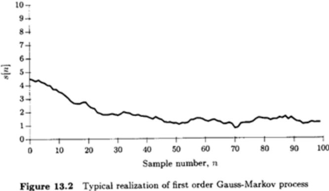
• A simple model to specify the correlation : first-order Gauss-Markov process
  $s[n]=as[n-1]+u[n],\;n\geq0$
  • $u[n]$ : WGN with variance
  • $\sigma^2_u$ : driving or excitation noise
  • $s[-1]\sim\mathcal{N}(\mu_s,\sigma^2_s)$, independent of $u[n],\;n\geq0$
  • $s[n]$ : output of LTI system driven by $u[n]$
    
• Dynamical or state model : The current output ($s[n]$) depends only on the state of the system at the previous time ($s[n-1]$) and the current input ($u[n]$)
• In general,
  $s[n]=a^{n+1}s[-1]+\sum^n_{k=0}a^ku[n-k]$
  linear with $s[-1]$ and $u[n-k]$'s : Gaussian random process

---

• Gaussian random process
  $E(s[n])=a^{n+1}\mu_s$
  • The covariance between $s[m]$ and $s[n]$ assuming $m\geq n$ is
    $c_s[m, n] = \mathbb{E}\left[(s[m] - \mathbb{E}(s[m]))(s[n] - \mathbb{E}(s[n]))\right]\\[0.2cm] = \mathbb{E}\left[\left(a^{m+1}(s[-1] - \mu_s) + \sum_{k=0}^m a^k u[m-k]\right) \left(a^{n+1}(s[-1] - \mu_s) + \sum_{l=0}^n a^l u[n-l]\right)\right]\\[0.2cm] = a^{m+n+2}\sigma_s^2 + \sum_{k=0}^m \sum_{l=0}^n a^{k+l} \mathbb{E}(u[m-k] u[n-l])\\[0.2cm] = a^{m+n+2}\sigma_s^2 + \sigma_u^2 \sum_{k=0}^m a^{2k} a^{n-m}\\[0.2cm] E(u[m-k]u[n-l])=\sigma^2_u\delta[l-(n-m+k)]\\[0.2cm] = a^{m+n+2}\sigma_s^2 + \sigma_u^2 a^{n-m} \sum_{k=0}^{n-m} a^{2k}\\[0.2cm] \rightarrow c_s[m, n] = c_s[n, m] \quad \text{for } m < n$
• $s[n]$ is not WSS, but as $n\rightarrow \infty,\;\text{for }|a|<1$
  $\mathbb{E}(s[n]) \rightarrow 0, \quad r_{ss}[k] = c_s[m, n] \Big|_{m-n=k} \rightarrow \frac{\sigma_u^2 a^k}{1 - a^2}$
  $s[n]$ can be WSS for $n>0$ if we choose $\mu_s,\sigma^2_s$ carefully
• Recursive form
  $\mathbb{E}(s[n]) = a \mathbb{E}(s[n-1]) + \mathbb{E}(u[n]) \\ = a \mathbb{E}(s[n-1])$

(mean and variance propagation eqns)

• $p$th-order Gauss-Markov process
  $s[n] = -\sum_{k=1}^p a[k] s[n-k] + u[n]$

• state vector
  $s[n] = \begin{bmatrix} s[n-p+1] \\ s[n-p+2] \\ \vdots \\ s[n] \end{bmatrix} = \begin{bmatrix} 0 & 1 & 0 & \cdots & 0 \\ 0 & 0 & 1 & \cdots & 0 \\ \vdots & \vdots & \vdots & \ddots & \vdots \\ -a[p] & -a[p-1] & -a[p-2] & \cdots & -a[1] \end{bmatrix} \begin{bmatrix} s[n-p] \\ s[n-p+1] \\ \vdots \\ s[n-1] \end{bmatrix} +\begin{bmatrix} 0 \\ 0 \\ \vdots \\ 1 \end{bmatrix} u[n]$

---

• Generalized vector Gauss-Markov model
  $s[n]=As[n-1]+Bu[n],\;n\geq0$
  • State model, $A$ : state transition matrix $p\times p$
    • $B : p\times r$ matrix
    • $s[n] : p\times 1$ signal vector
    • $u[n] : r\times 1$ driving noise vector
  • Statiscal assumptions
    1. $u[n]$ is a vector WGN sequence, i.e. $u[n]$ is a sequence of uncorrelated jointly Gaussian vectors with $E[u[n]]=0$
       As a result,
       $E(u[m]u^T[n])=0,\;m\neq n\\[0.2cm] E(u[n]u^T[n])=Q$
    2. $s[-1]\sim \mathcal{N}(\mu_s,C_s)$ and $s[-1]$ independent of $u[n],\;n\geq0$
• Two DC power supplies example
  • Two DC power supply outputs which are independent (in a functional sense)
    $s_1[n] = a_1 s_1[n-1] + u_1[n], \quad s_2[n] = a_2 s_2[n-1] + u_2[n]$

• All random variables are independent of each other
  $s[n] = \begin{bmatrix} s_1[n] \\ s_2[n] \end{bmatrix} = \begin{bmatrix} a_1 & 0 \\ 0 & a_2 \end{bmatrix} \begin{bmatrix} s_1[n-1] \\ s_2[n-1] \end{bmatrix} +\begin{bmatrix}1 & 0 \\0 & 1\end{bmatrix}\begin{bmatrix} u_1[n] \\ u_2[n] \end{bmatrix}$

---

• Statistical properties of the vector Gauss-Markov model
  $s[n]=A^{n+1}s[-1]+\sum^n_{k=0}A^kBu[n-k]$
  where $A^0=I \rightarrow$ Gaussian random process, $E(s[n])=A^{n+1}E(s[-1])=A^{n+1}\mu_s$
  $c_s[m, n] = \mathbb{E}\left[(s[m] - \mathbb{E}(s[m]))(s[n] - \mathbb{E}(s[n]))^T\right]$

---

• The eigenvalues of $A$ must be less than $1$ magnitude for a stable process
  • If so, as $n\rightarrow \infty$
    $E(s[n])=A^{n+1}\mu_s\rightarrow 0$
  • It can be shown that $A^{n+1}C_s{A^{n+1}}^T\rightarrow 0$ so that
    $C[n]\rightarrow C=\sum^\infty_{k=0}A^kBQB^T{A^k}^T$
  • Also, for steady state, $C[n]=C[n-1]=C$ in recursion,
    $C=ACA^T+BQB^T$
  • It is also possible to make $A$, $B$ and $Q$ time-dependent

---

Scalar Kalman Filter

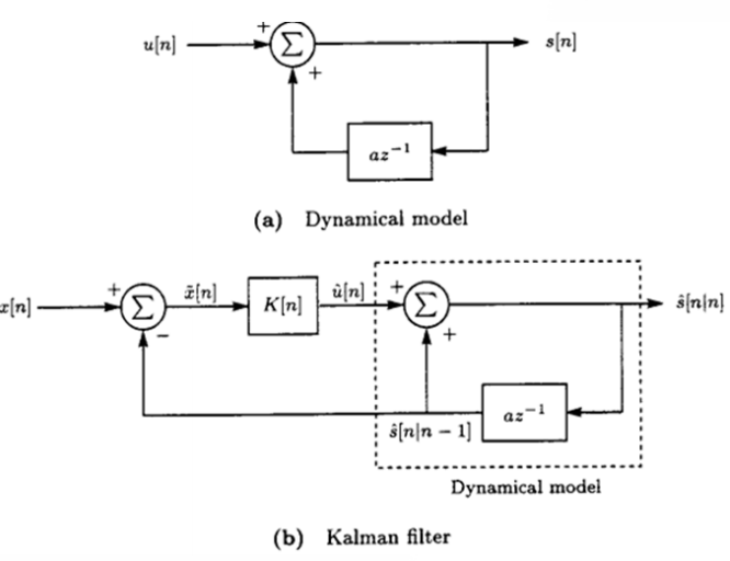
• Data Model(scalar Gauss-Markov signal model)
  • $s[n]=as[n-1]+u[n],\;n\geq0\text{ (scalar state equation)}$
  • $x[n]=s[n]+w[n]\text{ (scalar observation equation)}$
• Assumptions
  • $u[n]\sim\mathcal{N}(0, \sigma^2_u),\;u[n]$ and $u[m]$ indep. for $m\neq n$
  • $w[n]\sim\mathcal{N}(0, \sigma^2_n),\;w[n]$ and $w[m]$ indep. for $m \neq n$ (variance can change with time)
  • $s[-1]\sim\mathcal{N}(0, \sigma^2_s)$, independent of $u[n],\;w[n],\;n\geq0$
• Sequential MMSE estimator that estimates $s[n]$ based on $x[0],x[1],\cdots,x[n]$ as $n$ increases : filtering
• Goal : recursively compute
  $\hat s[n|n]=E(s[n]|x[0],x[1],\cdots,x[n])$
• Minimize $E[s[n]-\hat s[n|n])^2] \rightarrow \hat s[n|n]=E(s[n]|x[0],x[1],\cdots,x[n])$
• Since $\theta=s[n]$ and $\text{x}=[x[0]\;\cdots\;x[n]]^T$ are jointly Gaussian
  (linear, identical to LMMSE estimator)
  $\hat s[n|n]=C_{\theta x}C^{-1}_{xx}\text{x}$
• For non-Gaussian case, it is still a LMMSE estimator
  $\rightarrow$ similar to sequential LMMSE estimation with vector space approach
• Let's denote $X[n]=[x[0]\;\cdots\;x[n]]^T$ to avoid confusion with vector observations
  $\tilde x[n]=x[n]-\hat x[n|n-1] \text{ : innovation}\\[0.2cm] \hat s[n|n]=E(s[n]|X[n-1],\tilde x[n])=E(s[n]|X[n-1])+E(s[n]|\tilde x[n])\\[0.2cm] \text{Orthogonalization}\\[0.2cm] =\hat s[n|n-1]+E(s[n]|\tilde x[n]) \; (*)$

---

• $\hat s[n|n-1]=E(as[n-1]+u[n]|X[n-1])=a\hat s[n-1|n-1]$
• $E(s[n]|\tilde x[n])$ : MMSE estimator, linear because of the zero mean assumptions
  $\mathbb{E}(s[n] | \tilde{x}[n]) = K[n] \tilde{x}[n] = K[n] \left( x[n] - \hat{x}[n | n-1] \right)$

---

• To evaluate $K[n]$, we have

1. $E[s[n](x[n]-\hat s[n|n-1])]=E[(s[n]-\hat s[n|n-1])(x[n]-\hat s[n|n-1])]$
   since $\hat s[n|n-1]$, a linear combination of $s[n-k]$, are orthogonal to error
2. $E[w[n](s[n]-\hat s[n|n-1])] =0$
   $K[n] = \frac{\mathbb{E}\left((s[n] - \hat{s}[n | n-1])(x[n] - \hat{s}[n | n-1])\right)}{\mathbb{E}\left((s[n] - \hat{s}[n | n-1] + w[n])^2\right)}$

where $M[n|n-1]$ is MSE when $s[n]$ is estimated based on previous data

---

• Summary
  • Prediction : $\hat s[n|n-1]=a\hat s[n-1|n-1]$
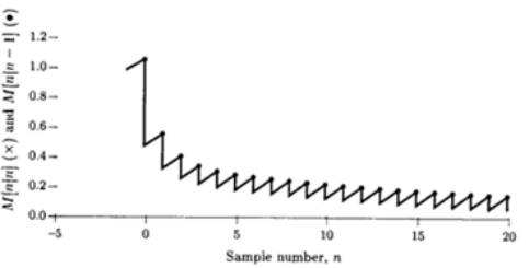
  • Minimum Prediction MSE : $M[n|n-1]=a^2M[n-1|n-1]+\sigma^2_u$
  • Kalman Gain : $K[n]=\frac{M[n|n-1]}{M[n|n-1]+\sigma^2_n}$
  • Correction : $\hat s[n|n]=\hat s[n|n-1]+K[n](x[n]-\hat s[n|n-1])$
  • Minimum MSE : $M[n|n]=(1-K[n])M[n|n-1]$
• The derivation was with $\mu_s=0$, but the same equations result for $\mu_s \neq 0$
  • Initialization : $\hat s[-1|-1]=E(s[-1])=\mu_s$ and $M[-1|-1]=\sigma^2_s$
  • $K[n](x[n]-\hat s[n|n-1])$ can be thought as the estimator of $u[n]$
  • $\hat s[n|n] = a\hat s[n-1|n-1] + \hat u[n]$ where $\hat u[n]=K[n](x[n]-\hat s[n|n-1])$
    

---

Scalar Kalman Filter - Properties

1. Kalman filter is an extension to the sequential MMSE estimator (LMMSE for non-Gaussian) where the unknown parameter evolves in time according to the dynamic model. The sequential MMSE estimator is a special case of Kalman filter for $a=1$ and $\sigma^2_u=0$
2. No matrix inversions are required
3. The Kalman filter is a time varying filter
   $\hat s[n|n]=a\hat s[n-1|n-1]+K[n](x[n]-a\hat s[n-1|n-1])\\[0.2cm] =a(1-K[n])\hat s[n-1|n-1] + K[n]x[n]$
   : first order recursive filter with time varying coefficients
4. The Kalman filter provides its own performance measure. Minimum Bayesian MSE is computed as an integral part of the estimator
5. The prediction stage increases the error, while the correction stage decreases it. The minimum prediction MSE and the minimum MSE is shown
   
6. Predictions is an integral part of the Kalman filter. One-step prediction is already computed. If we desire the best two-step prediction, we can let $\sigma^2_n \rightarrow \infty$ implying $x[n]$ is noisy enough to ignore and obtain $\hat s[n+1|n-1] = \hat s[n+1|n]=a\hat s[n|n]=a\hat s[n|n-1]=a^2\hat s[n-1|n-1]$
   It can be generalized to the $l$ step predictor
7. The Kalman filter is driven by the uncorrelated innovation sequence and in steady-state can also by viewed as a whitening filter
   $\hat s[n|n]=a\hat s[n-1|n-1]+K[n](x[n]-\hat s[n|n-1])$
   If we think the innovation
   $\tilde x[n]=x[n]-\hat s[n|n-1]$
   as the Kalman filter output, it is a whitening filter
8. For non-Gaussian case, it is still the optimum LMMSE estimator

---

Vector Kalman Filter

• The $p \times 1$ signal vector $s[n]$ evolves in time according to the Gauss-Markov model
  $x[n]=A[n]s[n-1]+B[n]u[n],\;n\geq0$
• $A[n],B[n]$ are known matrices of dimension $p \times p$ and $p \times r$, respectively
• $u[n]$ has the PDF $u[n]\sim\mathcal{N}(0, Q[n])$ are independent
  $E(u[m]u^T[n])=0,$ for $m \neq n\;(u[n]$ is vector WGN)
• $s[-1]$ has the PDF $s[-1]\sim\mathcal{N}(\mu_s,C_s)$ and is independent of $u[n]$

---

• The $M\times 1$ observation vectors $\text{x}[n]$ are modeled by the Bayesian linear model
  $\text{x}[n]=H[n]s[n]+w[n],\;n\geq0$
  • $H[n]$ is a known $M\times p$ observations matrix (which may be time varying)
  • $w[n]$ is an $M \times 1$ observation noise vector with PDF
  • $w[n]\sim\mathcal{N}(0, C[n])$ are independent
    $E(w[m]w^T[n])=0,\;\text{for }m\neq n$
    (If $C[n]$ does not depend on $n$, $w[n]$ would be vector WGN)

---

• The MMSE estimator of $s[n]$ based on $x[0],x[1],\cdots,x[n]$
  $\hat s[n|n]=E(s[n]|x[0],x[1],\cdots,x[n])$
• Prediction
  • Minimum Prediction MSE Matrix ($p \times p$)
    $M[n|n-1]=A[n]M[n-1|n-1]A^T[n]+B[n]Q[n]B^T[n]$
  • Kalman Gain Matrix ($p\times M$) :
    $M[n|n]=(I-K[n]H[n])M[n|n-1]$
• The recursion is initialized by $\hat s[-1|-1]=\mu_s$, and $M[-1|-1]=C_s$

All Content has been written based on lecture of Prof. eui-seok.Hwang in GIST(Detection and Estimation)