Difference between Detection and Estimation

• Estimation : Continuous set of hypotheses(almost always wrong - minimize error instead)
• Detection : Discrete set of hypotheses(right or wrong)
• Classical : Hypotheses/parameters are fixed, non-random
• Bayesian : Hypotheses/parameters are treated as random variables with assumed priors

---

Overview

• Theory of hypothesis testing
• Simple hypothesis testing problem with completely known PDF
• Complicated hypothesis testing problem with unknown PDF
  • Primary approaches :
    • Classical approach based on the Neyman-Pearson theorem
    • Bayesian approach based on minimization of the Bayes risk

---

Mathematical Detection Problem

• Binary Hypothesis Test
  • Noise only hypothesis vs. signal present hypothesis(deterministic signals)
    $\mathcal{H}_0: x[n] = w[n], \quad \text{null hypothesis} \\ \mathcal{H}_1: x[n] = s[n] + w[n], \quad \text{alternative hypothesis}$
  • Example of the DC level in noise $(A=1)$
    • $s[n]=A=1$
    • $w[n]$ : zero mean Gaussian process $\sim\mathcal{N}(0, \sigma^2)$
    • $p(x[0];\mathcal{H}_0)=\frac{1}{\sqrt{2\pi\sigma^2}}\exp\left[-\frac{1}{2\sigma^2}x[0]^2\right]$
    • $p(x[0];\mathcal{H}_1)=\frac{1}{\sqrt{2\pi\sigma^2}}\exp\left[-\frac{1}{2\sigma^2}(x[0]-1)^2\right]$

---

Neyman-Pearson Theorem

• Reasonable approach
  $\mathcal{H}_1:x[0]>1/2\\\mathcal{H}_0:\text{otherwise}$
• Type 1 error : decide $\mathcal{H}_1$ when $\mathcal{H}_0$ is true(false alarm)
  $\rightarrow$ Probability of false alarm, $P_{FA} =P(\mathcal{H}_1;\mathcal{H}_0)$
• Type 2 error : decide $\mathcal{H}_0$ when $\mathcal{H}_1$ is true (miss)
  $\rightarrow$ Probability of miss $P_M=P(\mathcal{H}_0;\mathcal{H}_1)$
  $\rightarrow$ Probability of detection,
  $P_D=P(\mathcal{H}_1;\mathcal{H}_1)=1-P(\mathcal{H}_0;\mathcal{H}_1)=1-P_M$
  It is not possible to reduce both error probabilities simultaneously

Neyman-Pearson Test

• Maximize $P_D=P(\mathcal{H}_1;\mathcal{H}_1)$ subject to the constraint $P_{FA}=P(\mathcal{H}_1;\mathcal{H}_0)=\alpha$
• Example of the DC level in noise
  $A = 1, \, \sigma^2 = 1 \quad \text{(standard normal)} \\[0.2cm] P_{FA} = P(\mathcal{H}_1; \mathcal{H}_0) = \Pr(x[0] > \gamma; \mathcal{H}_0) = \int_{\gamma}^\infty \frac{1}{\sqrt{2\pi}} \exp\left(-\frac{1}{2}t^2\right) dt = Q(\gamma) \\[0.2cm] P_{FA} = 10^{-3} \rightarrow \gamma' = 3 \\[0.2cm] P_D = P(\mathcal{H}_1; \mathcal{H}_1) = \Pr(x[0] > \gamma; \mathcal{H}_1) \\[0.2cm] = \int_{\gamma'}^\infty \frac{1}{\sqrt{2\pi}} \exp\left(-\frac{1}{2}(t-1)^2\right) dt = Q(\gamma' - 1) = Q(2) = 0.023\\[0.2cm] \text{Prob of Detection}$
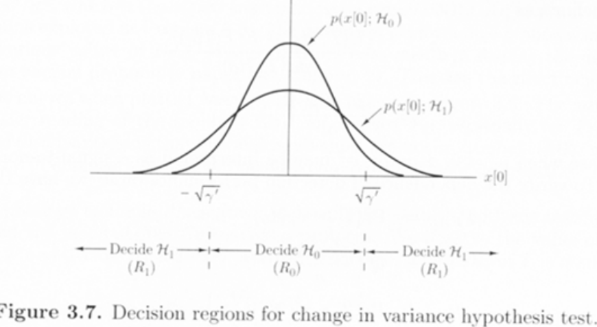
• Detector : decide $\mathcal{H}_0$ or $\mathcal{H}_1$ given $\text{x}=\{x[0],\cdots,x[n-1]\}$
• Decision region
  $R_1=\{\text{x}:\text{decide }\mathcal{H}_1 \text{ or reject }\mathcal{H}_0\}\\[0.2cm] R_0=\{\text{x}:\text{decide }\mathcal{H}_0 \text{ or reject }\mathcal{H}_1\}$
  • $R_0 \cup R_1=R^N$ (data space)
  • $P_{FA}=\int_{R_1}p(\text{x};\mathcal{H}_0)d\text{x}=\alpha$ : significance level or size
  • $P_D=\int_{R_1}p(\text{x};\mathcal{H}_1)d\text{x}$ : power of the test
• Neyman-Pearson Theorem
  To maximize $P_D$ for a given $P_{FA} = \alpha$, decide $\mathcal{H}_1$ if
  $L(\text{x})=\frac{p(\text{x};\mathcal{H}_1)}{p(\text{x};\mathcal{H}_0)}>\gamma$
  where the threshold $\gamma$ is found from
  $P_{FA}=\int_{\{\text{x}:L(\text{x})>\gamma\}}p(\text{x};\mathcal{H}_0)d\text{x}=\alpha$
  • $L(\text{x})=\frac{p(\text{x};\mathcal{H}_1)}{p(\text{x};\mathcal{H}_0)}$ : likelihood ratio : Likelihood ratio test(LRT)

Neyman-Pearson Therorem - Proof

• Using Lagrangian multipliers,
  $F=P_D+\lambda(P_{FA}-\alpha)=\int_{R_1}p(\text{x};\mathcal{H}_1)d\text{x}+\lambda\left(\int_{R_1}p(\text{x};\mathcal{H}_0)d\text{x}-\alpha\right)\\[0.2cm] =\int_{R_1}(p(\text{x};\mathcal{H}_1)+\lambda p(\text{x};\mathcal{H}_0))d\text{x}-\lambda\alpha$
• To maximize $F$, we should include $\text{x}$ in $\mathcal{H}_1$ if the integrand is positive, i.e., if
  $p(\text{x};\mathcal{H}_1)+\lambda p(\text{x};\mathcal{H}_0) >0$
  • decide $\mathcal{H}_1$ if $\frac{p(\text{x};\mathcal{H}_1)}{p(\text{x};\mathcal{H}_0)} > -\lambda$ ($\lambda$ should be negative)
  • decide $\mathcal{H}_1$ if $\frac{p(\text{x};\mathcal{H}_1)}{p(\text{x};\mathcal{H}_0)}>\gamma$ ($\gamma$ is found from $P_{FA}=\alpha$

---

• DC level in noise $(A=1)$ with $P_{FA}=10^{-3}$
  $\frac{p(x; \mathcal{H}_1)}{p(x; \mathcal{H}_0)} = \frac{\exp\left[-\frac{1}{2}(x[0] - 1)^2\right]}{\exp\left[-\frac{1}{2}x^2[0]\right]} \rightarrow \gamma \rightarrow \exp\left(x[0] - \frac{1}{2}\right) > \gamma \\[0.2cm] P_{FA} = \Pr\left\{\exp\left(x[0] - \frac{1}{2}\right) > \gamma; \mathcal{H}_0\right\} = 10^{-3}$
• Let $\gamma'=\ln\gamma+1/2$, then
  $P_{FA} = \int_{\gamma}^\infty \frac{1}{\sqrt{2\pi}} \exp\left(-\frac{1}{2}t^2\right) dt = 10^{-3} \rightarrow \gamma' = 3 \\[0.2cm] P_D = \Pr\{x[0] > 3; \mathcal{H}_1\} = \int_{3}^\infty \frac{1}{\sqrt{2\pi}} \exp\left(-\frac{1}{2}(t-1)^2\right) dt = 0.023$
• If $P_{FA}=0.5$
  $P_{FA} = \int_{\gamma'}^\infty \frac{1}{\sqrt{2\pi}} \exp\left(-\frac{1}{2}t^2\right) dt = 0.5 \implies \gamma' = 0 \\[0.2cm] P_D = \int_{0}^\infty \frac{1}{\sqrt{2\pi}} \exp\left(-\frac{1}{2}(t-1)^2\right) dt = Q(-1) = 1 - Q(1) = 0.84$

---

• Example of the DC level in WGN
  $\mathcal{H}_0: x[n] = w[n], \quad n = 0, 1, \dots, N-1 \\[0.2cm] \mathcal{H}_1: x[n] = s[n] + w[n], \quad n = 0, 1, \dots, N-1 \\[0.2cm] w[n] \sim \mathcal{N}(0, \sigma^2), \quad S[n] = A \\[0.2cm] \mathcal{H}_0: \mu = 0 \\[0.2cm] \mathcal{H}_1: \mu = A1$
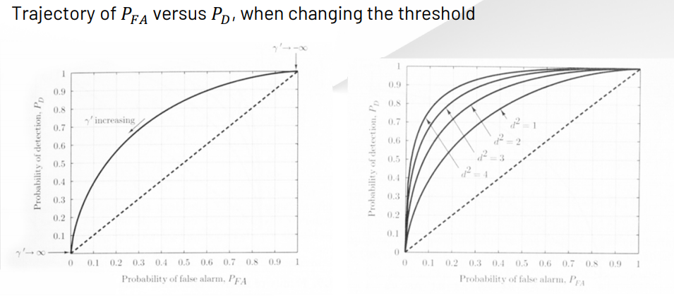
• Decide $\mathcal{H}_1$ if
  $\frac{\exp\left[-\frac{1}{2\sigma^2} \sum_{n=0}^{N-1} (x[n] - A)^2\right]}{\exp\left[-\frac{1}{2\sigma^2} \sum_{n=0}^{N-1} x^2[n]\right]} > \gamma \\[0.2cm] \rightarrow -\frac{1}{2\sigma^2} \left(-2A \sum_{n=0}^{N-1} x[n] + N A^2\right) > \ln \gamma\\[0.2cm] \frac{A}{\sigma^2} \sum_{n=0}^{N-1} x[n] > \ln \gamma + \frac{N A^2}{2\sigma^2} \\[0.2cm] \frac{1}{N} \sum_{n=0}^{N-1} x[n] > \frac{\sigma^2}{N A} \ln \gamma + \frac{A}{2} = \gamma' \\[0.2cm] T(\mathbf{x}) = \frac{1}{N} \sum_{n=0}^{N-1} x[n], \quad T(\mathbf{x}) \sim \begin{cases} \mathcal{N}\left(0, \frac{\sigma^2}{N}\right), & \text{under } \mathcal{H}_0 \\[0.2cm] \mathcal{N}\left(A, \frac{\sigma^2}{N}\right), & \text{under } \mathcal{H}_1 \end{cases} \\[0.2cm] P_{FA} = \Pr(T(\mathbf{x}) > \gamma'; \mathcal{H}_0) = Q\left(\frac{\gamma'}{\sqrt{\sigma^2 / N}}\right) \rightarrow \gamma' = \sqrt{\frac{\sigma^2}{N}} Q^{-1}(P_{FA}) \\[0.2cm] P_D = \Pr(T(\mathbf{x}) > \gamma'; \mathcal{H}_1) = Q\left(\frac{\gamma' - A}{\sqrt{\sigma^2 / N}}\right) \\[0.2cm] \rightarrow P_D = Q\left(\sqrt{\frac{N}{\sigma^2}} Q^{-1}(P_{FA}) - \sqrt{\frac{N}{\sigma^2}} A\right) = Q\left(Q^{-1}(P_{FA}) - \sqrt{\frac{N A^2}{\sigma^2}}\right)$

---

• Deflection coefficient $d$ is defined for a test statistic $T$ as,
  $d^2=\frac{(E(T;\mathcal{H}_1)-E(T;\mathcal{H}_0))^2}{\text{var}(T;\mathcal{H}_0)}$
  • Useful in characterizing the performance of a detector
  • Usually, the larger the deflection coefficient, the easier it is to differentiate between the two signals, and thus the better the detection performance
• For the mean shifted Gaussian problem,
  $T \sim \begin{cases} \mathcal{N}(\mu_0, \sigma^2), & \text{under } \mathcal{H}_0 \\[0.2cm] \mathcal{N}(\mu_1, \sigma^2), & \text{under } \mathcal{H}_1 \end{cases} \quad \rightarrow \quad d^2 = \frac{(\mu_1 - \mu_0)^2}{\sigma^2} \\[0.2cm] P_D = Q\left(Q^{-1}(P_{FA}) - \sqrt{d^2}\right)$

---

• Example of change in variance

  $\mathcal{H}_0 : x[n] \sim \mathcal{N}(0, \sigma_0^2), \quad n = 0, 1, \dots, N-1 \\[0.2cm] \mathcal{H}_1 : x[n] \sim \mathcal{N}(0, \sigma_1^2), \quad n = 0, 1, \dots, N-1 \\[0.2cm] \sigma_1^2 > \sigma_0^2$

  

• NP Test : Decide $\mathcal{H}_1$ if

  $\frac{\frac{1}{(2\pi \sigma_1^2)^{N/2}} \exp\left[-\frac{1}{2\sigma_1^2} \sum_{n=0}^{N-1} x^2[n]\right]} {\frac{1}{(2\pi \sigma_0^2)^{N/2}} \exp\left[-\frac{1}{2\sigma_0^2} \sum_{n=0}^{N-1} x^2[n]\right]} > \gamma \\[0.2cm] -\frac{1}{2} \left(\frac{1}{\sigma_1^2} - \frac{1}{\sigma_0^2}\right) \sum_{n=0}^{N-1} x^2[n] > \ln \gamma + \frac{N}{2} \ln \frac{\sigma_1^2}{\sigma_0^2} \\[0.2cm] \frac{1}{N} \sum_{n=0}^{N-1} x^2[n] > (\frac{2}{N} \ln \gamma + \ln \frac{\sigma_1^2}{\sigma_0^2} )\bigg/ \left(\frac{1}{\sigma_0^2} - \frac{1}{\sigma_1^2}\right) = \gamma'$

---

• Test statistic and sufficient statistic
  • Assume that we observe $\text{x}=[x[0]\;\cdots\;x[n]]^T$ with a PDF that is parameterized by $\theta,p(\text{x};\theta)$
    $\mathcal{H}_0:\theta=\theta_0\\[0.2cm] \mathcal{H}_1:\theta=\theta_1$
  • By Neyman-Fisher factorization theorem
    $p(\text{x};\theta)=g(T(\text{x}),\theta)h(\text{x}), \text{where }T(\text{x}) \text{ is a sufficient statistic for }\theta$
  • The NP test becomes
    $\frac{p(\text{x};\theta_1)}{p(\text{x};\theta_0)}>\gamma\rightarrow\frac{g(T(\text{x}),\theta_1)}{g(T(\text{x}),\theta_0)}>\gamma$
    However, a single sufficient statistic doesn't always exist

Receiver Operating Characteristics(ROC)

Bayes Risk

• $P(\mathcal{H}_i),\;i=0,1$ : prior probability of each hypothesis
• $C_{ij}$ : cost of deciding $\mathcal{H}_i$ when $\mathcal{H}_j$ is true
• Bayes risk
  $R=E(C)=\sum^1_{i=0}\sum^1_{j=0}C_{ij}P(\mathcal{H}_i|\mathcal{H}_j)P(\mathcal{H}_j)$
• Usually $C_{00}=C_{11}=0$
• If $C_{ij}=1-\delta_{ij}\rightarrow R=P_e$ (minimum probability of error)
  $P_e=P(\mathcal{H}_0|\mathcal{H}_1)P(\mathcal{H}_1)+P(\mathcal{H}_1|\mathcal{H}_0)P(\mathcal{H}_0)$

  $P_e$ = Probability of miss + Probability of False alarm

• Bayes risk detector
  $R = C_{00} P(\mathcal{H}_0) \int_{R_0} p(x|\mathcal{H}_0) dx + C_{01} P(\mathcal{H}_1) \int_{R_0} p(x|\mathcal{H}_1) dx \\[0.2cm] \quad + C_{10} P(\mathcal{H}_0) \int_{R_1} p(x|\mathcal{H}_0) dx + C_{11} P(\mathcal{H}_1) \int_{R_1} p(x|\mathcal{H}_1) dx \\[0.2cm] = C_{00} P(\mathcal{H}_0) + C_{01} P(\mathcal{H}_1) \\[0.2cm] \quad + \int_{R_1} \left[(C_{10} P(\mathcal{H}_0) - C_{00} P(\mathcal{H}_0)) p(x|\mathcal{H}_0)\right] dx \\[0.2cm] \quad + \int_{R_1} \left[(C_{11} P(\mathcal{H}_1) - C_{01} P(\mathcal{H}_1)) p(x|\mathcal{H}_1)\right] dx$
• Including $\text{x}$ in $R_1$ if the integrand is negative
  • Decide $\mathcal{H}_1$ if
    $(C_{10}-C_{00})P(\mathcal{H}_0)p(\text{x}|\mathcal{H}_0) <(C_{01}-C_{11})P(\mathcal{H}_1)p(\text{x}|\mathcal{H}_1)$
  • Decide $\mathcal{H}_1$ if
    $\text{LRT Bayesian }\frac{p(\text{x}|\mathcal{H}_1)}{p(\text{x}|\mathcal{H}_0)}>\frac{(C_{10}-C_{00})P(\mathcal{H}_0)}{(C_{01}-C_{11})P(\mathcal{H}_1)}=\gamma$
    • In Classical $\gamma=\alpha=P_{FA}$

---

• Example of DC Level in WGN (Minimum probaility of error criterion)
  $\mathcal{H}_0:x[n]=w[n],\;n=0,1,\cdots,N-1\\[0.2cm] \mathcal{H}_1:x[n]=s[n]+w[n],\;n=0,1,\cdots,N-1\\[0.2cm] w[n]\sim\mathcal{N}(0,\sigma^2), \text{WGN},P(\mathcal{H}_0)=P(\mathcal{H}_1)=1/2$
• Minimizing $P_e$ : Deicide $\mathcal{H}_1$ if
  $L(\text{x})=\frac{p(\text{x}|\mathcal{H}_1)}{p(\text{x}|\mathcal{H}_0)}>\frac{(C_{10}-C_{00})P(\mathcal{H}_0)}{(C_{01}-C_{11})P(\mathcal{H}_1)}=1\\[0.2cm] =\frac{(1-0)1/2}{(1-0)1/2}=1$
• Decide $\mathcal{H}_1$ if
  $\bar x>\frac{A}{2}\text{ (the same as NP criterion except the threshold)}\\[0.2cm] \bar x\sim\begin{cases} \mathcal{N}(0,\sigma^2/N) \text{ under }\mathcal{H}_0\\ \mathcal{N}(A,\sigma^2/N)\text{ under }\mathcal{H}_1 \end{cases}\\[0.2cm] P_e=\frac{1}{2}\left[P(\mathcal{H}_0|\mathcal{H}_1)+P(\mathcal{H}_1|\mathcal{H}_0)\right]\\[0.2cm] =\frac{1}{2}\left[\Pr\{\bar x<A/2|\mathcal{H}_1\} + \Pr\{\bar x > A/2|\mathcal{H}_0\}\right]\\[0.2cm] =\frac{1}{2}\left[\left(1-Q\left(\frac{A/2-A}{\sqrt{\sigma^2/N}}\right)\right)+Q\left(\frac{A/2}{\sqrt{\sigma^2/N}}\right)\right]\\[0.2cm] =Q\left(\frac{A/2}{\sqrt{\sigma^2/N}}\right)=Q\left(\sqrt{\frac{NA^2}{4\sigma^2}}\right)$

  Large $A$ and large $\sigma^2$ : good

Multiple Hypothesis Testing

• $M$ hypothesis instead of 2. (Ex. QPSK) : a.k.a. classification or discrimination
  • Bayes risk
    $R=\sum^{M-1}_{i=0}\sum^{M-1}_{j=0}C_{ij}P(\mathcal{H}_i|\mathcal{H}_j)P(\mathcal{H}_j)$
  • Decision rule : Choose the hypothesis that minimizes
    $C_i(\text{x})=\sum^{M-1}_{j=0}C_{ij}P(\mathcal{H}_j|\text{x})\text{ over }i=0,1,\cdots M-1$
  • Decision rule to minimize $P_e$ : Minimize
    $C_i(\text{x})=\sum^{M-1}_{j=0}P(\mathcal{H}_j|\text{x})-P(\mathcal{H}_i|\text{x})$
    maximize $P(\mathcal{H}_i|\text{x})$ : maximum a posteriori probability(MAP) rule
    $\max_iP(\mathcal{H}_i|\text{x})=\max_iP(\text{x}|\mathcal{H}_i)P(\mathcal{H}_i) \rightarrow \text{ML rule if }P(\mathcal{H}_i) \text{ are all equal}$

    Maximum Likelihood

All Content has been written based on lecture of Prof. eui-seok.Hwang in GIST(Detection and Estimation)