Overview

Detection of a known signal in Gaussian noise

• NP criterion or Bayes risk criterion
• The test statistic is a linear function of the data due to the Gaussian noise assumption
• The detector resulted from these assumptions is called the matched filter

---

Matched Filters

• Detecting a known deterministic signal $s[n],\;n=0,1,\cdots,N-1$ in white Gaussian noise Neyman-Pearson criterion will be used
• Bayesian risk criterion will result in the same test statistic; only the threshold differs
• Binary hypothesis
  $\mathcal{H}_0:x[n]=w[n],\quad n=0,1,\cdots,N-1\\[0.2cm] \mathcal{H}_1:x[n]=s[n]+w[n],\quad n=0,1,\cdots,N-1\\[0.2cm] s[n]:\text{known signal},\;w[n]:\text{WGN with variance }\sigma^2\\[0.2cm] \text{ACF }r_{ww}[k]=E(w[n]w[n+k])=\sigma^2\delta[k]$
• NP detector : decide $\mathcal{H}_1$ if
  $L(\text{x})=\frac{p(\text{x};\mathcal{H}_1)}{p(\text{x};\mathcal{H}_0)}>\gamma\\[0.2cm] \rightarrow\frac{\ln p(\text{x};\mathcal{H}_1)}{\ln p(\text{x};\mathcal{H}_0)}>\ln \gamma$

---

---

• decide $\mathcal{H}_1$ if
  $\sum_{n=0}^{N-1} x[n] s[n] - \frac{1}{2\sigma^2} \sum_{n=0}^{N-1} s^2[n] > \ln \gamma \\[0.2cm] \rightarrow T(x) = \sum_{n=0}^{N-1} x[n] s[n] > \sigma^2 \ln \gamma + \frac{1}{2} \sum_{n=0}^{N-1} s^2[n] = \gamma'$

---

• Ex) Damped exponential in WGN
  $s[n]=r^n,0<r<1\\[0.2cm] \rightarrow T(\text{x})=\sum^{N-1}_{n=0}x[n]r^n$
• Correlator (replica-correlator)
  $T(\text{x})=\sum^{N-1}_{n=0}x[n]s[n]$
• Alternatively, if $x[n]$ is an input signal to a finite impulse response (FIR) filter with impulse response $h[n]$ which is nonzero for $n=0,1,\cdots,N-1$, the output becomes
  $y[n]=\sum^n_{k=0}h[n-k]x[k]$
• If we let $h[n]=s[N-1-n],\;n=0,1,\cdots,N-1$ then,
  $y[n]=\sum^n_{k=0}s[N-1-(n-k)]x[k]\\[0.2cm] y[N-1]=\sum^{N-1}_{k=0} s[k]x[k] \rightarrow \text{Matched Filter}$

---

• In the frequency domain

  $y[n]=\int^{\frac{1}{2}}_{-\frac{1}{2}}H(f)X(f)\exp(j2\pi fn)df\\[0.2cm] H(f),X(f):\text{discrete-time Fourier transform of }h[n],x[n]\\[0.2cm] h[n]=s[N-1-n]\rightarrow H(f)=S^*(f)\exp[-j2\pi f(N-1)]\\[0.2cm] y[n]=\int^{\frac{1}{2}}_{-\frac{1}{2}}S^*(f)X(f)\exp(j2\pi f(n-(N-1))df\rightarrow y[N-1]=\int^{\frac{1}{2}}_{-\frac{1}{2}}S^*(f) X(f)df$
  • Matched filter emphasizes the band with more signal power
  • When the noise is absent, the matched filter output is just the signal energy

• A filter which maximizes the SNR at the output ($\eta$) of the filter

  $\eta = \frac{\mathbb{E}^2\left(y[N-1]; \mathcal{H}_1\right)}{\text{var}\left(y[N-1]; \mathcal{H}_1\right)} = \frac{\left(\sum_{k=0}^{N-1} h[N-1-k] s[k]\right)^2} {\mathbb{E}\left[\left(\sum_{k=0}^{N-1} h[N-1-k] w[k]\right)^2\right]}$

• Let $\mathbf{s} = [s[0] \, s[1] \, \dots \, s[N-1]]^T$

• $\mathbf{h} = [h[N-1] \, h[N-2] \, \dots \, h[0]]^T$

• $\mathbf{w} = [w[0] \, w[1] \, \dots \, w[N-1]]^T$

  $\text{then} \quad \eta = \frac{(\mathbf{h}^T \mathbf{s})^2}{\mathbb{E}[(\mathbf{h}^T \mathbf{w})^2]} = \frac{(\mathbf{h}^T \mathbf{s})^2}{\mathbf{h}^T \mathbb{E}(\mathbf{w} \mathbf{w}^T) \mathbf{h}} = \frac{(\mathbf{h}^T \mathbf{s})^2}{\mathbf{h}^T \sigma^2 \mathbf{I} \mathbf{h}} = \frac{1}{\sigma^2} \frac{(\mathbf{h}^T \mathbf{s})^2}{\mathbf{h}^T \mathbf{h}}$

• By the Cauchy-Schwarz inequality

  $(\text{h}^T\text{s})^2\leq(\text{h}^T\text{h})(\text{s}^T\text{s})$

  with equality if and only if $\text{h}=c\text{s}$

• Then

  $\eta\leq\frac{1}{\sigma^2}\text{s}^T\text{s}$

  with equality if and only if $\text{h}=c\text{s}$

• The maximum SNR is attained for

  $h[N-1-n]=s[n]\\[0.2cm] \text{or }h[n]=s[N-1-n],\quad n=0,1,\cdots,N-1$

• For WGN, the NP criterion and the maximum SNR criterion lead to the same matched filter

• For non-Gaussian case, NP detector is not linear

---

Performance of matched filter

($P_D$ for a given $P_{FA}$)

• $\mathcal{H}_1$ if
  $T(\text{x})=\sum^{N-1}_{n=0}x[n]s[n]>\gamma^2\\[0.2cm] T(\text{x})\text{ is Gaussian}\\[0.2cm] \mathbb{E}(T; \mathcal{H}_0) = \mathbb{E}\left(\sum_{n=0}^{N-1} w[n] s[n]\right) = 0, \\[0.2cm] \mathbb{E}(T; \mathcal{H}_1) = \mathbb{E}\left(\sum_{n=0}^{N-1} (s[n] + w[n]) s[n]\right) = \sum_{n=0}^{N-1} s^2[n] \triangleq \mathcal{E} \\[0.2cm] \text{var}(T; \mathcal{H}_0) = \text{var}\left(\sum_{n=0}^{N-1} w[n] s[n]\right) = \sum_{n=0}^{N-1} \text{var}(w[n]) s^2[n] = \sigma^2 \sum_{n=0}^{N-1} s^2[n] = \sigma^2 \mathcal{E} \\[0.2cm] \text{var}(T; \mathcal{H}_1) = \text{var}(T; \mathcal{H}_0)$

---

The test statistic

• Thus
  $P_{FA} = \Pr\{T > \gamma'; \mathcal{H}_0\} = Q\left(\frac{\gamma'}{\sqrt{\sigma^2 \mathcal{E}}}\right) \\[0.2cm] P_D = \Pr\{T > \gamma'; \mathcal{H}_1\} = Q\left(\frac{\gamma' - \mathcal{E}}{\sqrt{\sigma^2 \mathcal{E}}}\right) = Q\left(Q^{-1}(P_{FA}) - \sqrt{\frac{\mathcal{E}}{\sigma^2}}\right)$

---

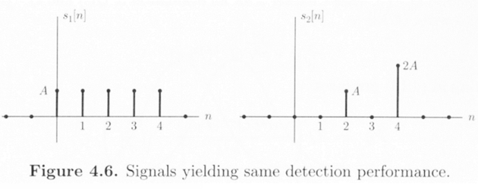
• The shape of the signal does not affect the detection performance
• Only the ENR matters
• But the signal shape affects the performance when the noise is colored
  

---

Generalized Matched Filters

Correlated noise : $\text{w}\sim \mathcal{N}(0,\text{C})$

• If the noise is WSS, $[\text{C}]_{mn}=r_{ww}[m-n]$ : a symmetric Toeplitz matrix
• If the noise is nonstationary, $\text{C}$ will be arbitrary covariance matrix
  $p(x; \mathcal{H}_1) = \frac{1}{(2\pi)^{N/2} \sqrt{\det \mathbf{C}}} \exp\left(-\frac{1}{2} (x - s)^T \mathbf{C}^{-1} (x - s)\right) \\[0.2cm] p(x; \mathcal{H}_0) = \frac{1}{(2\pi)^{N/2} \sqrt{\det \mathbf{C}}} \exp\left(-\frac{1}{2} x^T \mathbf{C}^{-1} x\right)$
• LRT : decide $\mathcal{H}_1$ if
  $l(x) = \ln \frac{p(x; \mathcal{H}_1)}{p(x; \mathcal{H}_0)} > \ln \gamma, \\[0.2cm] l(x) = x^T \mathbf{C}^{-1} s - \frac{1}{2} s^T \mathbf{C}^{-1} s$
• $T(\text{x})=\text{x}^T\mathbf{C}^{-1}\text{s}>\gamma'$ : generalized matched filter
• If we let $s''=C^{-1}s,\;T(\text{x})=\text{x}^Ts''$ : correlation with modified signal

---

Prewhitening

• For any $\text{C}$(positive definite), it can be shown that $\text{C}^{-1}$ exists and is also positive definite
  $\rightarrow C^{-1}=D^TD$ where $D$ is a nonsingular prewhitening matrix
  $T(\text{x})=\text{x}^TC^{-1}s=\text{x}^TD^TDs=\text{x}'^Ts'\\[0.2cm] \text{where }\text{x}'=D\text{x},\;s'=Ds$
• Prewhitening : $\text{w}'=D\text{w}$ becomes WGN
  as $C_{\text{w}'}=E(\text{w}'\text{w}'^T)=DCD^T=I$
• If the length $N$ is large and the noise is WSS
  $T(\text{x})=\int^{1/2}_{-1/2}\frac{X(f)S^*(f)}{P_{\text{w}\text{w}}(f)}df$
  where $P_{\text{w}\text{w}(f)}$ is the PSD of the noise (Power Spectral Density)

---

Performance of generalized matched filter

---

• Example of signal design for uncorrelated noise with unequal variances
  $\mathbf{C}^{-1} = \text{diag}\left(\frac{1}{\sigma_0^2}, \frac{1}{\sigma_1^2}, \dots, \frac{1}{\sigma_{N-1}^2}\right) \rightarrow s^T \mathbf{C}^{-1} s = \sum_{n=0}^{N-1} \frac{s^2[n]}{\sigma_n^2}$
  • We want to maximize $d^2=\text{s}^TC^{-1}\text{s}$ subject to the constraint
    $\sum_{n=0}^{N-1} s^2[n] = \mathcal{E}$
  • By using Lagrangian multipliers
    $F = \sum_{n=0}^{N-1} \frac{s^2[n]}{\sigma_n^2} + \lambda \left(\mathcal{E} - \sum_{n=0}^{N-1} s^2[n]\right) \\[0.2cm] \frac{\partial F}{\partial s[k]} = \frac{2s[k]}{\sigma_k^2} - 2\lambda s[k] = 2s[k] \left(\frac{1}{\sigma_k^2} - \lambda\right) = 0, \quad k = 0, 1, \dots, N-1$

---

• Assuming all the $\sigma^2_n$ are different, we can have
  $\left(\frac{1}{\sigma^2_k}-\lambda\right)=0$
  for at most one $k$
• Let $j$ be the index that satisfies
  $\left(\frac{1}{\sigma^2_j}-\lambda\right)=0$
• Then $s[k]=0$ for $k\neq j$
  $\text{s}^TC^{-1}\text{s}=\frac{s^2[j]}{\sigma^2_j}=\frac{\mathcal{E}}{\sigma^2_j}$
  $\rightarrow$ choose $j$ for which $\sigma^2_j$ is minimum

---

For an arbitrary noise covariance matrix

• The signal is chosen by maximizing $\text{s}^TC^{-1}\text{s}$ subject to the fixed energy constraint $s^Ts=\mathcal{E}$
  $F = s^T \mathbf{C}^{-1} s + \lambda \left(\mathcal{E} - s^T s\right) \\[0.2cm] \frac{\partial F}{\partial s} = 2 \mathbf{C}^{-1} s - 2\lambda s = 0 \\[0.2cm] \rightarrow \mathbf{C}^{-1} s = \lambda s \quad \rightarrow \quad s \text{ is an eigenvector of } \mathbf{C}^{-1} \\[0.2cm] s^T \mathbf{C}^{-1} s = s^T \lambda s = \lambda \mathcal{E}$
  • $\text{s}$ is eigenvector of $C^{-1}$ corresponding to the largest eigenvalue $\lambda$
  • Alternatively, $Cs=\frac{1}{\lambda}s$
    $s$ is the eigenvector of $C$ corresponding to the minimum eigenvalue $\lambda$

---

Example of signal design for colored noise

• Eigenvalues
  $(C-\lambda_iI)\text{v}=0\rightarrow\lambda_1=1+\rho,\;\lambda_2=1-\rho$
• Eigenvectors
  $\text{v}_1=\left[\begin{matrix}1/\sqrt{2}\\1/\sqrt{2}\end{matrix}\right],\;\text{v}_2=\left[\begin{matrix}1/\sqrt{2}\\-1/\sqrt{2}\end{matrix}\right]$
• Assuming $\rho>0,\text{s}=\sqrt{\mathcal{E}}\text{v}_2=\sqrt{\mathcal{E}/2}\left[\begin{matrix}1\\-1\end{matrix}\right]$
  $\rightarrow T(x) = x^T \mathbf{C}^{-1} s = x^T \mathbf{C}^{-1} \sqrt{\mathcal{E}} v_2 = \sqrt{\mathcal{E}} x^T \frac{1}{\lambda_2} v_2 = \frac{\sqrt{\mathcal{E}/2}}{1 - \rho} \left(x[0] - x[1]\right)$
• Since $s[1]=-s[0]$, the signal contribution in $(x[0]-x[1])$ will not be cancelled
  $d^2 = s^T \mathbf{C}^{-1} s = \mathcal{E} v_2^T \mathbf{C}^{-1} v_2 = \mathcal{E} v_2^T \frac{1}{\lambda_2} v_2 \\[0.2cm] = \frac{\mathcal{E}}{\lambda_2} = \frac{\mathcal{E}}{1 - \rho}$
• For a large data record and WSS noise,
  $d^2 = \int_{-1/2}^{1/2} \frac{|S(f)|^2}{P_{ww}(f)} df$
  concentrate signal energy to the band where the noise PSD is minimum

---

Multiple Signals

Sonar/radar systems : detection of a known signal in noise
Communication systems : signal is there, but we should decide which signal it is

Binary case

• Minimum probability of error criterion & equal prior probabilities
  $\mathcal{H}_0 : x[n] = s_0[n] + w[n], \quad n = 0, 1, \cdots, N-1 \\[0.2cm] \mathcal{H}_1 : x[n] = s_1[n] + w[n], \quad n = 0, 1, \cdots, N-1 \\[0.2cm] s_0[n], s_1[n] : \text{known deterministic signals,} \quad w[n] : \text{WGN with variance } \sigma^2$
• Decide $\mathcal{H}_1$ if
  $\frac{p(x | \mathcal{H}_1)}{p(x | \mathcal{H}_0)} > \gamma = \frac{(C_{10} - C_{00})P(\mathcal{H}_0)}{(C_{01} - C_{11})P(\mathcal{H}_1)} = 1, \\[0.2cm] p(x | \mathcal{H}_i) = \frac{1}{(2\pi\sigma^2)^{N/2}} \exp \left[ -\frac{1}{2\sigma^2} \sum_{n=0}^{N-1} \left(x[n] - s_i[n]\right)^2 \right]$
• Decide $\mathcal{H}_i$ for which
  $D_i^2 = \sum_{n=0}^{N-1} \left(x[n] - s_i[n]\right)^2 \text{ is minimum.} \\[0.2cm] \rightarrow \text{minimum distance criterion} \\[0.2cm] D_i^2 = \left(x - s_i\right)^T \left(x - s_i\right) = \|x - s_i\|^2 \\[0.2cm] \text{: squared Euclidean distance} \\[0.2cm] \rightarrow \text{Choose the hypothesis whose signal vector is closest to } x \\[0.2cm] \text{Decide } \mathcal{H}_i \text{ for which} \\[0.2cm] T_i(x) = \sum_{n=0}^{N-1} x[n]s_i[n] - \frac{1}{2} \sum_{n=0}^{N-1} s_i^2[n] = \sum_{n=0}^{N-1} x[n]s_i[n] - \frac{1}{2}\mathcal{E}_i$

---

Performance

---

• Example of phase shift keying(PSK)
  $s_0[n] = A \cos 2 \pi f_0 n \\[0.2cm] s_1[n] = A \cos (2 \pi f_0 n + \pi) = -A \cos 2 \pi f_0 n \\[0.2cm] \rho_s = \frac{s_1^T s_0}{\bar{\mathcal{E}}} = -1 \implies P_e = Q \left( \sqrt{\frac{\bar{\mathcal{E}}}{\sigma^2}} \right)$
• Example of frequency shift keying(FSK)
  $s_0[n] = A \cos 2 \pi f_0 n, \quad n = 0, \cdots, N-1 \\[0.2cm] s_1[n] = A \cos 2 \pi f_1 n, \quad n = 0, \cdots, N-1 \\[0.2cm] \bullet \ \text{If } |f_1 - f_0| \gg \frac{1}{2N}, \ \text{the signals are approximately orthogonal.} \\[0.2cm] \rho_s = 0 \implies P_e = Q \left( \sqrt{\frac{\bar{\mathcal{E}}}{2 \sigma^2}} \right)$

---

M-ARY Case

$M$ signals $s_0[n],s_1[n],\cdots,s_{M-1}[n]$ with equal prior probabilities

• Choose $\mathcal{H}_i$ for which $p(\text{x}|\mathcal{H}_i)$ is maximum
• Choose $\mathcal{H}_k$ if
  $T_k(\mathbf{x}) = \sum_{n=0}^{N-1} x[n] s_k[n] - \frac{1}{2} \mathcal{E}_k \\[0.2cm] \text{is the maximum statistic of } \{T_0(\mathbf{x}), T_1(\mathbf{x}), \cdots, T_{M-1}(\mathbf{x})\}.$

Performance

• In general, difficult to evaluate the probability of error
• Assume that the signals are orthogonal and have equal energies $\mathcal{E}_i=\mathcal{E}$(for simplicity)
  $\text{cov}(T_i, T_j; \mathcal{H}_i) = E \left( \sum_{n=0}^{N-1} w[n] s_i[n] \sum_{n=0}^{N-1} w[n] s_j[n] \right) \\[0.2cm] = \sum_{m=0}^{N-1} \sum_{n=0}^{N-1} E(w[m] w[n]) s_i[m] s_j[n] \\[0.2cm] = \sigma^2 \sum_{n=0}^{N-1} s_i[n] s_j[n] = 0 \quad \text{for } i \neq j \\[0.2cm] P_e = \sum_{i=0}^{M-1} \text{Pr} \{T_i < \max(T_0, \cdots, T_{i-1}, T_{i+1}, \cdots, T_{M-1}) \; | \; \mathcal{H}_i\} P(\mathcal{H}_i) \\[0.2cm] = \text{Pr} \{T_0 < \max(T_1, T_2, \cdots, T_{M-1}) \; | \; \mathcal{H}_0\}.$
• Conditioned on $\mathcal{H}_0$
  $T_i(\mathbf{x}) = \sum_{n=0}^{N-1} x[n] s_i[n] - \frac{1}{2} \mathcal{E}_i \sim \begin{cases} \mathcal{N} \left( \frac{1}{2} \mathcal{E}_i, \sigma^2 \mathcal{E} \right), & \text{for } i = 0 \\[0.2cm] \mathcal{N} \left( -\frac{1}{2} \mathcal{E}_i, \sigma^2 \mathcal{E} \right), & \text{for } i \neq 0 \end{cases} \\[0.4cm] P_e = 1 - \text{Pr} \{ T_0 > \max(T_1, T_2, \cdots, T_{M-1}) \; | \; \mathcal{H}_0 \} \\[0.2cm] = 1 - \text{Pr} \{ T_1 < T_0, T_2 < T_0, \cdots, T_{M-1} < T_0 \; | \; \mathcal{H}_0 \} \\[0.2cm] = 1 - \int_{-\infty}^\infty \text{Pr} \{ T_1 < t, T_2 < t, \cdots, T_{M-1} < t \; | \; T_0 = t, \mathcal{H}_0 \} p_{T_0}(t) \, dt \\[0.2cm] = 1 - \int_{-\infty}^\infty \prod_{i=1}^{M-1} \text{Pr} \{ T_i < t \; | \; \mathcal{H}_0 \} p_{T_0}(t) \, dt.$
  $= 1 - \int_{-\infty}^\infty \Phi^{M-1} \left( \frac{t + \frac{1}{2} \mathcal{E}}{\sqrt{\sigma^2 \mathcal{E}}} \right) \frac{1}{\sqrt{2\pi \sigma^2 \mathcal{E}}} \exp \left[ -\frac{1}{2\sigma^2 \mathcal{E}} \left( t - \frac{1}{2} \mathcal{E} \right)^2 \right] dt \\[0.4cm] = 1 - \int_{-\infty}^\infty \Phi^{M-1}(u) \frac{1}{\sqrt{2\pi}} \exp \left[ -\frac{1}{2} \left( u - \sqrt{\frac{\mathcal{E}}{\sigma^2}} \right)^2 \right] du \\[0.4cm] \text{where } \Phi(\cdot) \text{ is the CDF of } \mathcal{N}(0,1) \text{ random variable.}$

All Content has been written based on lecture of Prof. eui-seok.Hwang in GIST(Detection and Estimation)