Overview
So far, detection under
Neyman-Pearson criteria ( max P D P_D P D P F A = P_{FA}= P F A = ) ) ) P F A P_{FA} P F A Minimize Bayesian risk (assign costs to decisions, have priors of the different hypothesis) : likelihood ratio test, threshold set by priors+costs
minimum probability of error = maximum a posteriori detection
maximum likelihood detection = minimum probability of error with equal priors
Known deterministic signals in Gaussian noise : correlators
Random signals : estimator-correlators, energy detectors
All assume knowledge of p ( x ; H 0 ) p(x;\mathcal{H}_0) p ( x ; H 0 ) p ( x ; H 1 p(x;\mathcal{H}_1 p ( x ; H 1
What if don't know the distribution of x x x
What if under hypothesis 0, distribution is in some set, and under hypothesis 1, this distribution lies in another set - can we distinguish between these two?
Composite Hypothesis Testing
Composite Hypothesis Testing
Signal and / or noise PDF have unknown parameters i.e. noise var., exact carrier freq., signal var.,
Composite hypothesis test : must accommodate unknown parameters
cf. simple hypothesis test : the PDFs are completely known
Ex) DC level in WGN with unknown amplitude A > 0 A>0 A > 0 H 0 : x [ n ] = w [ n ] vs H 1 : x [ n ] = A + w [ n ] , n = 0 , 1 , … , N − 1 ∙ NP test: decide H 1 if p ( x ; A , H 1 ) p ( x ; H 0 ) = exp [ − 1 2 σ 2 ∑ n = 0 N − 1 ( x [ n ] − A ) 2 ] exp [ − 1 2 σ 2 ∑ n = 0 N − 1 x 2 [ n ] ] > γ , T ( x ) = 1 N ∑ n = 0 N − 1 x [ n ] > σ 2 N A ln γ + A 2 = γ ′ . \mathcal{H}_0 : x[n] = w[n] \quad \text{vs} \quad \mathcal{H}_1 : x[n] = A + w[n], \quad n = 0, 1, \dots, N-1 \\[0.2cm] \bullet \; \text{NP test: decide } \mathcal{H}_1 \text{ if} \\[0.2cm] \frac{p(x; A, \mathcal{H}_1)}{p(x; \mathcal{H}_0)} = \frac{\exp \left[ -\frac{1}{2\sigma^2} \sum_{n=0}^{N-1} (x[n] - A)^2 \right]}{\exp \left[ -\frac{1}{2\sigma^2} \sum_{n=0}^{N-1} x^2[n] \right]} > \gamma, \\[0.2cm] T(x) = \frac{1}{N} \sum_{n=0}^{N-1} x[n] > \frac{\sigma^2}{NA} \ln \gamma + \frac{A}{2} = \gamma'. H 0 : x [ n ] = w [ n ] vs H 1 : x [ n ] = A + w [ n ] , n = 0 , 1 , … , N − 1 ∙ NP test: decide H 1 if p ( x ; H 0 ) p ( x ; A , H 1 ) = exp [ − 2 σ 2 1 ∑ n = 0 N − 1 x 2 [ n ] ] exp [ − 2 σ 2 1 ∑ n = 0 N − 1 ( x [ n ] − A ) 2 ] > γ , T ( x ) = N 1 n = 0 ∑ N − 1 x [ n ] > N A σ 2 ln γ + 2 A = γ ′ .
Can we implement this detector without knowledge of the exact value of A A A
The test statistic does not depend on A A A γ ′ \gamma' γ ′ T ( x ) ∼ { N ( 0 , σ 2 N ) under H 0 N ( A , σ 2 N ) under H 1 P F A = Pr ( T ( x ) > γ ′ ; H 0 ) = Q ( γ ′ σ 2 / N ) , P D = Pr ( T ( x ) > γ ′ ; H 1 ) = Q ( γ ′ − A σ 2 / N ) , γ ′ = σ 2 N Q − 1 ( P F A ) : independent of A P D = Q ( Q − 1 ( P F A ) − N A 2 σ 2 ) : depend on the value of A 1 N ∑ n = 0 N − 1 x [ n ] > σ 2 N Q − 1 ( P F A ) yields the highest P D for any value of A > 0. T(x) \sim \begin{cases} \mathcal{N}\left(0, \frac{\sigma^2}{N}\right) & \text{under } \mathcal{H}_0 \\ \mathcal{N}\left(A, \frac{\sigma^2}{N}\right) & \text{under } \mathcal{H}_1 \end{cases} \\[0.2cm] P_{FA} = \Pr(T(x) > \gamma'; \mathcal{H}_0) = Q\left(\frac{\gamma'}{\sqrt{\sigma^2 / N}}\right), \\[0.2cm] P_D = \Pr(T(x) > \gamma'; \mathcal{H}_1) = Q\left(\frac{\gamma' - A}{\sqrt{\sigma^2 / N}}\right), \\[0.2cm] \gamma' = \sqrt{\frac{\sigma^2}{N}} Q^{-1}(P_{FA}) : \text{independent of } A \\[0.2cm] P_D = Q\left(Q^{-1}(P_{FA}) - \sqrt{\frac{NA^2}{\sigma^2}}\right) : \text{depend on the value of } A \\[0.2cm] \frac{1}{N} \sum_{n=0}^{N-1} x[n] > \sqrt{\frac{\sigma^2}{N}} Q^{-1}(P_{FA}) \; \text{yields the highest } P_D \; \text{for any value of } A > 0. T ( x ) ∼ ⎩ ⎪ ⎨ ⎪ ⎧ N ( 0 , N σ 2 ) N ( A , N σ 2 ) under H 0 under H 1 P F A = Pr ( T ( x ) > γ ′ ; H 0 ) = Q ( σ 2 / N γ ′ ) , P D = Pr ( T ( x ) > γ ′ ; H 1 ) = Q ( σ 2 / N γ ′ − A ) , γ ′ = N σ 2 Q − 1 ( P F A ) : independent of A P D = Q ( Q − 1 ( P F A ) − σ 2 N A 2 ) : depend on the value of A N 1 n = 0 ∑ N − 1 x [ n ] > N σ 2 Q − 1 ( P F A ) yields the highest P D for any value of A > 0 .
Uniformly Most Powerful(UMP) test
If − ∞ < A < ∞ -\infty<A<\infty − ∞ < A < ∞ A A A
The hypothesis testing problem → \rightarrow → H 0 : A = 0 H 1 : A > 0 (one-sided test → UMP exists.) H 0 : A = 0 H 1 : A ≠ 0 (two-sided test → UMP test does not exist.) \begin{aligned} &\mathcal{H}_0 : A = 0 \\[0.2cm] &\mathcal{H}_1 : A > 0 \quad \text{(one-sided test → UMP exists.)} \\[0.5cm] &\mathcal{H}_0 : A = 0 \\[0.2cm] &\mathcal{H}_1 : A \neq 0 \quad \text{(two-sided test → UMP test does not exist.)} \end{aligned} H 0 : A = 0 H 1 : A > 0 (one-sided test → UMP exists.) H 0 : A = 0 H 1 : A = 0 (two-sided test → UMP test does not exist.)
When a UMP test does not exist, we have to implement suboptimal tests
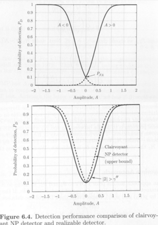
The optimal NP test, which is unrealizable, can provide an upper bound of the performance
Clairvoyant Detector : a detector assuming perfect knowledge of an unknown parameter to design the NP detector
Example of DC Level in WGN with unknown amplitude − ∞ < A < ∞ -\infty<A<\infty − ∞ < A < ∞
Clairvoyant detector : decide H 1 \mathcal{H}_1 H 1 1 N ∑ n = 0 N − 1 x [ n ] > γ + ′ for A > 0 , 1 N ∑ n = 0 N − 1 x [ n ] < γ − ′ for A < 0. \frac{1}{N} \sum_{n=0}^{N-1} x[n] > \gamma'_+ \quad \text{for } A > 0, \\[0.2cm] \frac{1}{N} \sum_{n=0}^{N-1} x[n] < \gamma'_- \quad \text{for } A < 0. N 1 n = 0 ∑ N − 1 x [ n ] > γ + ′ for A > 0 , N 1 n = 0 ∑ N − 1 x [ n ] < γ − ′ for A < 0 . Under H 0 \mathcal{H}_0 H 0 x ˉ ∼ N ( 0 , σ 2 N ) \bar x\sim\mathcal{N}(0,\frac{\sigma^2}{N}) x ˉ ∼ N ( 0 , N σ 2 ) P F A = Pr { x ˉ > γ + ′ ; H 0 } = Q ( γ + ′ σ 2 N ) if A > 0 , P F A = Pr { x ˉ < γ − ′ ; H 0 } = 1 − Q ( γ − ′ σ 2 N ) = Q ( − γ − ′ σ 2 N ) if A < 0. P_{FA} = \Pr\{\bar{x} > \gamma'_+; \mathcal{H}_0\} = Q\left(\frac{\gamma'_+}{\sqrt{\frac{\sigma^2}{N}}}\right) \quad \text{if } A > 0, \\[0.2cm] P_{FA} = \Pr\{\bar{x} < \gamma'_-; \mathcal{H}_0\} = 1 - Q\left(\frac{\gamma'_-}{\sqrt{\frac{\sigma^2}{N}}}\right) = Q\left(\frac{-\gamma'_-}{\sqrt{\frac{\sigma^2}{N}}}\right) \quad \text{if } A < 0. P F A = Pr { x ˉ > γ + ′ ; H 0 } = Q ⎝ ⎜ ⎛ N σ 2 γ + ′ ⎠ ⎟ ⎞ if A > 0 , P F A = Pr { x ˉ < γ − ′ ; H 0 } = 1 − Q ⎝ ⎜ ⎛ N σ 2 γ − ′ ⎠ ⎟ ⎞ = Q ⎝ ⎜ ⎛ N σ 2 − γ − ′ ⎠ ⎟ ⎞ if A < 0 .
For a constant P F A P_{FA} P F A γ − ′ = − γ + ′ \gamma'_- =-\gamma'_+ γ − ′ = − γ + ′
Under H 1 \mathcal{H}_1 H 1 x ˉ ∼ ( A , σ 2 N ) \bar x\sim\left(A,\frac{\sigma^2}{N}\right) x ˉ ∼ ( A , N σ 2 ) P D = Q ( γ + ′ − A σ 2 N ) = Q ( Q − 1 ( P F A ) − N A 2 σ 2 ) , if A > 0 , P D = 1 − Q ( γ − ′ − A σ 2 N ) = Q ( − γ − ′ + A σ 2 N ) = Q ( Q − 1 ( P F A ) − N A 2 σ 2 ) , if A < 0. P_D = Q\left(\frac{\gamma'_+ - A}{\sqrt{\frac{\sigma^2}{N}}}\right) = Q\left(Q^{-1}(P_{FA}) - \sqrt{\frac{NA^2}{\sigma^2}}\right), \quad \text{if } A > 0, \\[0.2cm] P_D = 1 - Q\left(\frac{\gamma'_- - A}{\sqrt{\frac{\sigma^2}{N}}}\right) = Q\left(\frac{-\gamma'_- + A}{\sqrt{\frac{\sigma^2}{N}}}\right) = Q\left(Q^{-1}(P_{FA}) - \sqrt{\frac{NA^2}{\sigma^2}}\right), \quad \text{if } A < 0. P D = Q ⎝ ⎜ ⎛ N σ 2 γ + ′ − A ⎠ ⎟ ⎞ = Q ( Q − 1 ( P F A ) − σ 2 N A 2 ) , if A > 0 , P D = 1 − Q ⎝ ⎜ ⎛ N σ 2 γ − ′ − A ⎠ ⎟ ⎞ = Q ⎝ ⎜ ⎛ N σ 2 − γ − ′ + A ⎠ ⎟ ⎞ = Q ( Q − 1 ( P F A ) − σ 2 N A 2 ) , if A < 0 .
A candidate detector : decide H 1 \mathcal{H}_1 H 1 ∣ 1 N ∑ n = 0 N − 1 x [ n ] ∣ > r ′ ′ |\frac{1}{N}\sum^{N-1}_{n=0}x[n]|>r'' ∣ N 1 ∑ n = 0 N − 1 x [ n ] ∣ > r ′ ′ P D = Q ( Q − 1 ( P F A 2 ) − N A 2 σ 2 ) + Q ( Q − 1 ( P F A 2 ) + N A 2 σ 2 ) . P_D = Q\left(Q^{-1}\left(\frac{P_{FA}}{2}\right) - \sqrt{\frac{NA^2}{\sigma^2}}\right) + Q\left(Q^{-1}\left(\frac{P_{FA}}{2}\right) + \sqrt{\frac{NA^2}{\sigma^2}}\right). P D = Q ( Q − 1 ( 2 P F A ) − σ 2 N A 2 ) + Q ( Q − 1 ( 2 P F A ) + σ 2 N A 2 ) .
Composite Hypothesis Testing Approaches
Two major approaches
Bayesian approach
Requires prior knowledge of the unknown parameters
Requires multidimensional integration
Generalized likelihood ratio test(GLRT)
More popular due to the ease of implementation and less restricitive assumptions
Prior knowledge is not necessary
Bayesian approach
p ( x ; H 0 ) = ∫ p ( x ∣ θ 0 ; H 0 ) p ( θ 0 ) d θ 0 p ( x ; H 1 ) = ∫ p ( x ∣ θ 1 ; H 1 ) p ( θ 1 ) d θ 1 Decide H 1 if p ( x ; H 1 ) p ( x ; H 0 ) = ∫ p ( x ∣ θ 1 ; H 1 ) p ( θ 1 ) d θ 1 ∫ p ( x ∣ θ 0 ; H 0 ) p ( θ 0 ) d θ 0 > γ . p(x; \mathcal{H}_0) = \int p(x | \theta_0; \mathcal{H}_0) p(\theta_0) d\theta_0 \\[0.3cm] p(x; \mathcal{H}_1) = \int p(x | \theta_1; \mathcal{H}_1) p(\theta_1) d\theta_1 \\[0.3cm] \text{Decide } \mathcal{H}_1 \text{ if } \frac{p(x; \mathcal{H}_1)}{p(x; \mathcal{H}_0)} = \frac{\int p(x | \theta_1; \mathcal{H}_1) p(\theta_1) d\theta_1}{\int p(x | \theta_0; \mathcal{H}_0) p(\theta_0) d\theta_0} > \gamma. p ( x ; H 0 ) = ∫ p ( x ∣ θ 0 ; H 0 ) p ( θ 0 ) d θ 0 p ( x ; H 1 ) = ∫ p ( x ∣ θ 1 ; H 1 ) p ( θ 1 ) d θ 1 Decide H 1 if p ( x ; H 0 ) p ( x ; H 1 ) = ∫ p ( x ∣ θ 0 ; H 0 ) p ( θ 0 ) d θ 0 ∫ p ( x ∣ θ 1 ; H 1 ) p ( θ 1 ) d θ 1 > γ . Generalized Likelihood Ratio Test
The GLRT replaces the unknown parameters by their maximum likelihood estimators(MLEs)
There is no optimality associated with the GLRT, but it works well in practice
GLRT : Decide H 1 \mathcal{H}_1 H 1
L G ( x ) = p ( x ; θ ^ 1 , H 1 ) p ( x ; θ ^ 0 , H 0 ) > γ , where θ ^ i is the MLE of θ i assuming H i is true (maximizes p ( x ; θ ^ i , H i ) ) . L_G(x) = \frac{p(x; \hat{\theta}_1, \mathcal{H}_1)}{p(x; \hat{\theta}_0, \mathcal{H}_0)} > \gamma, \\[0.3cm] \text{where } \hat{\theta}_i \text{ is the MLE of } \theta_i \text{ assuming } \mathcal{H}_i \text{ is true (maximizes } p(x; \hat{\theta}_i, \mathcal{H}_i) \text{)}. L G ( x ) = p ( x ; θ ^ 0 , H 0 ) p ( x ; θ ^ 1 , H 1 ) > γ , where θ ^ i is the MLE of θ i assuming H i is true (maximizes p ( x ; θ ^ i , H i ) ) .
Example of DC Level in WGN with unknown amplitude - GLRT(θ 1 = A \theta_1=A θ 1 = A
H 0 : A = 0 H 1 : A ≠ 0 \mathcal{H}_0:A=0\\[0.2cm] \mathcal{H}_1:A\neq 0 H 0 : A = 0 H 1 : A = 0 A ^ = x ˉ → L G ( x ) = p ( x ; A ^ , H 1 ) p ( x ; H 0 ) > γ , L G ( x ) = exp [ − 1 2 σ 2 ∑ n = 0 N − 1 ( x [ n ] − x ˉ ) 2 ] exp [ − 1 2 σ 2 ∑ n = 0 N − 1 x 2 [ n ] ] , ln L G ( x ) = − 1 2 σ 2 ( ∑ n = 0 N − 1 x 2 [ n ] − 2 x ˉ ∑ n = 0 N − 1 x [ n ] + N x ˉ 2 ) − ∑ n = 0 N − 1 x 2 [ n ] , = − 1 2 σ 2 ( − 2 N x ˉ 2 + N x ˉ 2 ) = N x ˉ 2 2 σ 2 , → decide H 1 if ∣ x ˉ ∣ > γ ′ . \hat{A} = \bar{x} \rightarrow L_G(x) = \frac{p(x; \hat{A}, \mathcal{H}_1)}{p(x; \mathcal{H}_0)} > \gamma, \\[0.2cm] L_G(x) = \frac{\exp\left[-\frac{1}{2\sigma^2} \sum_{n=0}^{N-1} (x[n] - \bar{x})^2\right]}{\exp\left[-\frac{1}{2\sigma^2} \sum_{n=0}^{N-1} x^2[n]\right]}, \\[0.2cm] \ln L_G(x) = -\frac{1}{2\sigma^2} \left( \sum_{n=0}^{N-1} x^2[n] - 2\bar{x} \sum_{n=0}^{N-1} x[n] + N\bar{x}^2 \right) - \sum_{n=0}^{N-1} x^2[n], \\[0.2cm] = -\frac{1}{2\sigma^2} \left( -2N\bar{x}^2 + N\bar{x}^2 \right) = \frac{N\bar{x}^2}{2\sigma^2}, \\[0.2cm] \rightarrow \text{decide } \mathcal{H}_1 \text{ if } |\bar{x}| > \gamma'. A ^ = x ˉ → L G ( x ) = p ( x ; H 0 ) p ( x ; A ^ , H 1 ) > γ , L G ( x ) = exp [ − 2 σ 2 1 ∑ n = 0 N − 1 x 2 [ n ] ] exp [ − 2 σ 2 1 ∑ n = 0 N − 1 ( x [ n ] − x ˉ ) 2 ] , ln L G ( x ) = − 2 σ 2 1 ( n = 0 ∑ N − 1 x 2 [ n ] − 2 x ˉ n = 0 ∑ N − 1 x [ n ] + N x ˉ 2 ) − n = 0 ∑ N − 1 x 2 [ n ] , = − 2 σ 2 1 ( − 2 N x ˉ 2 + N x ˉ 2 ) = 2 σ 2 N x ˉ 2 , → decide H 1 if ∣ x ˉ ∣ > γ ′ .
Alternative form of GLRT
L G ( x ) = max θ 1 p ( x ; θ 1 , H 1 ) max θ 0 p ( x ; θ 0 , H 0 ) . L_G(x) = \frac{\max_{\theta_1} p(x; \theta_1, \mathcal{H}_1)}{\max_{\theta_0} p(x; \theta_0, \mathcal{H}_0)}. L G ( x ) = max θ 0 p ( x ; θ 0 , H 0 ) max θ 1 p ( x ; θ 1 , H 1 ) .
If the PDF under H 0 \mathcal{H}_0 H 0
L G ( x ) = max θ 1 p ( x ; θ 1 , H 1 ) p ( x ; H 0 ) = max θ 1 p ( x ; θ 1 , H 1 ) p ( x ; H 0 ) = max θ 1 L ( x ; θ 1 ) . L_G(x) = \frac{\max_{\theta_1} p(x; \theta_1, \mathcal{H}_1)}{p(x; \mathcal{H}_0)} = \max_{\theta_1} \frac{p(x; \theta_1, \mathcal{H}_1)}{p(x; \mathcal{H}_0)} = \max_{\theta_1} L(x; \theta_1). L G ( x ) = p ( x ; H 0 ) max θ 1 p ( x ; θ 1 , H 1 ) = θ 1 max p ( x ; H 0 ) p ( x ; θ 1 , H 1 ) = θ 1 max L ( x ; θ 1 ) .
Example of DC level in WGN with unknown amplitude and variance - GLRT
H 0 : A = 0 , σ 2 > 0 H 1 : A ≠ 0 , σ 2 > 0 , σ 2 : nuisance parameter . \mathcal{H}_0: A = 0, \, \sigma^2 > 0 \\ \mathcal{H}_1: A \neq 0, \, \sigma^2 > 0, \quad \sigma^2 : \text{nuisance parameter}. H 0 : A = 0 , σ 2 > 0 H 1 : A = 0 , σ 2 > 0 , σ 2 : nuisance parameter . (not of immediate interest, but must be accounted for the analysis of the parameters of interest)
GLRT : decide H 1 \mathcal{H}_1 H 1 L G ( x ) = p ( x ; A ^ , σ ^ 1 2 , H 1 ) p ( x ; σ ^ 0 2 , H 0 ) > γ , A ^ = x ˉ , σ ^ 0 2 = 1 N ∑ n = 0 N − 1 x 2 [ n ] , σ ^ 1 2 = 1 N ∑ n = 0 N − 1 ( x [ n ] − x ˉ ) 2 . p ( x ; A ^ , σ ^ 1 2 , H 1 ) = 1 ( 2 π σ ^ 1 2 ) N / 2 exp [ − 1 2 σ ^ 1 2 ∑ n = 0 N − 1 ( x [ n ] − A ^ ) 2 ] , p ( x ; σ ^ 0 2 , H 0 ) = 1 ( 2 π σ ^ 0 2 ) N / 2 exp [ − N 2 ] , 2 ln L G ( x ) = N ln σ ^ 0 2 σ ^ 1 2 . L_G(\mathbf{x}) = \frac{p(\mathbf{x}; \hat{A}, \hat{\sigma}_1^2, \mathcal{H}_1)}{p(\mathbf{x}; \hat{\sigma}_0^2, \mathcal{H}_0)} > \gamma, \\ \hat{A} = \bar{x}, \quad \hat{\sigma}_0^2 = \frac{1}{N} \sum_{n=0}^{N-1} x^2[n], \quad \hat{\sigma}_1^2 = \frac{1}{N} \sum_{n=0}^{N-1} \left( x[n] - \bar{x} \right)^2. \\ p(\mathbf{x}; \hat{A}, \hat{\sigma}_1^2, \mathcal{H}_1) = \frac{1}{(2\pi \hat{\sigma}_1^2)^{N/2}} \exp\left[ -\frac{1}{2\hat{\sigma}_1^2} \sum_{n=0}^{N-1} \left( x[n] - \hat{A} \right)^2 \right], \\ p(\mathbf{x}; \hat{\sigma}_0^2, \mathcal{H}_0) = \frac{1}{(2\pi \hat{\sigma}_0^2)^{N/2}} \exp\left[ -\frac{N}{2} \right], \\ 2 \ln L_G(\mathbf{x}) = N \ln \frac{\hat{\sigma}_0^2}{\hat{\sigma}_1^2}. L G ( x ) = p ( x ; σ ^ 0 2 , H 0 ) p ( x ; A ^ , σ ^ 1 2 , H 1 ) > γ , A ^ = x ˉ , σ ^ 0 2 = N 1 n = 0 ∑ N − 1 x 2 [ n ] , σ ^ 1 2 = N 1 n = 0 ∑ N − 1 ( x [ n ] − x ˉ ) 2 . p ( x ; A ^ , σ ^ 1 2 , H 1 ) = ( 2 π σ ^ 1 2 ) N / 2 1 exp [ − 2 σ ^ 1 2 1 n = 0 ∑ N − 1 ( x [ n ] − A ^ ) 2 ] , p ( x ; σ ^ 0 2 , H 0 ) = ( 2 π σ ^ 0 2 ) N / 2 1 exp [ − 2 N ] , 2 ln L G ( x ) = N ln σ ^ 1 2 σ ^ 0 2 .
Locally Most Powerful Detectors
For two-sided tests, a UMP test does not exist. For one-sided tests, a UMP test may not exist. One-sided test without any nuisance parameters
H 0 : θ = θ 0 , H 1 : θ > θ 0 \mathcal{H}_0:\theta=\theta_0,\;\mathcal{H}_1:\theta>\theta_0 H 0 : θ = θ 0 , H 1 : θ > θ 0 If we wish to test for values of θ \theta θ θ 0 \theta_0 θ 0 locally most powerful test exists
The LMP test does not guarantee the optimality if ∣ θ − θ 0 ∣ |\theta-\theta_0| ∣ θ − θ 0 ∣
NP test : decide H 1 \mathcal{H}_1 H 1 p ( x ; θ ) p ( x ; θ 0 ) > γ → ln p ( x ; θ ) − ln p ( x ; θ 0 ) > ln γ ln p ( x ; θ ) ≈ ln p ( x ; θ 0 ) + ∂ ln p ( x ; θ ) ∂ θ ∣ θ = θ 0 ( θ − θ 0 ) → ∂ ln p ( x ; θ ) ∂ θ ∣ θ = θ 0 > ln γ / ( θ − θ 0 ) = γ ′ , T LMP ( x ) = ∂ ln p ( x ; θ ) ∂ θ ∣ θ = θ 0 I ( θ 0 ) : scaled statistic . \frac{p(\mathbf{x}; \theta)}{p(\mathbf{x}; \theta_0)} > \gamma \quad \rightarrow \quad \ln p(\mathbf{x}; \theta) - \ln p(\mathbf{x}; \theta_0) > \ln \gamma \\ \ln p(\mathbf{x}; \theta) \approx \ln p(\mathbf{x}; \theta_0) + \left. \frac{\partial \ln p(\mathbf{x}; \theta)}{\partial \theta} \right|_{\theta = \theta_0} (\theta - \theta_0) \quad \\[0.2cm] \rightarrow \quad \left. \frac{\partial \ln p(\mathbf{x}; \theta)}{\partial \theta} \right|_{\theta = \theta_0} > \ln \gamma / (\theta - \theta_0) = \gamma', \\ T_\text{LMP}(\mathbf{x}) = \frac{\left. \frac{\partial \ln p(\mathbf{x}; \theta)}{\partial \theta} \right|_{\theta = \theta_0}}{\sqrt{I(\theta_0)}}: \text{scaled statistic}. p ( x ; θ 0 ) p ( x ; θ ) > γ → ln p ( x ; θ ) − ln p ( x ; θ 0 ) > ln γ ln p ( x ; θ ) ≈ ln p ( x ; θ 0 ) + ∂ θ ∂ ln p ( x ; θ ) ∣ ∣ ∣ ∣ ∣ θ = θ 0 ( θ − θ 0 ) → ∂ θ ∂ ln p ( x ; θ ) ∣ ∣ ∣ ∣ ∣ θ = θ 0 > ln γ / ( θ − θ 0 ) = γ ′ , T LMP ( x ) = I ( θ 0 ) ∂ θ ∂ l n p ( x ; θ ) ∣ ∣ ∣ ∣ θ = θ 0 : scaled statistic .
Example of correlation testing
2-D IID Gaussian vectors { x [ 0 ] , x [ 1 ] , … , x [ N − 1 ] } , x [ n ] = [ x 1 [ n ] x 2 [ n ] ] T \{\mathbf{x}[0], \mathbf{x}[1], \dots, \mathbf{x}[N-1]\}, \quad \mathbf{x}[n] = \begin{bmatrix} x_1[n] \\ x_2[n] \end{bmatrix}^T { x [ 0 ] , x [ 1 ] , … , x [ N − 1 ] } , x [ n ] = [ x 1 [ n ] x 2 [ n ] ] T x [ n ] ∼ N ( 0 , C ) , C = σ 2 [ 1 ρ ρ 1 ] , C − 1 = σ − 2 [ 1 1 − ρ 2 − ρ 1 − ρ 2 − ρ 1 − ρ 2 1 1 − ρ 2 ] H 0 : ρ = 0 , H 1 : ρ > 0 p ( x ; ρ ) = ∏ n = 0 N − 1 1 ( 2 π ) det 1 / 2 ( C ) exp ( − 1 2 x [ n ] T C − 1 x [ n ] ) ln p ( x ; ρ ) = − N 2 ln 2 π − N 2 ln σ 4 ( 1 − ρ 2 ) − 1 2 σ 2 ∑ n = 0 N − 1 x [ n ] T C 0 − 1 x [ n ] ∂ ln p ( x ; ρ ) ∂ ρ = N ρ 1 − ρ 2 − 1 2 σ 2 ∑ n = 0 N − 1 x [ n ] T ∂ C 0 − 1 ∂ ρ x [ n ] ∂ C 0 − 1 ∂ ρ = [ 2 ρ ( 1 − ρ 2 ) 2 − 1 + ρ 2 ( 1 − ρ 2 ) 2 − 1 + ρ 2 ( 1 − ρ 2 ) 2 2 ρ ( 1 − ρ 2 ) 2 ] ∂ ln p ( x ; ρ ) ∂ ρ ∣ ρ = 0 = − 1 σ 2 ∑ n = 0 N − 1 x T [ n ] [ 0 − 1 − 1 0 ] x [ n ] = ∑ n = 0 N − 1 x 1 [ n ] x 2 [ n ] σ 2 I ( ρ ) = N ( 1 + ρ 2 ) ( 1 − ρ 2 ) 2 ⟹ I ( 0 ) = N T L M P ( x ) = ∑ n = 0 N − 1 x 1 [ n ] x 2 [ n ] N σ 2 = N ρ ^ > γ ′ ρ ^ = 1 N ∑ n = 0 N − 1 x 1 [ n ] x 2 [ n ] σ 2 is an estimate of ρ , although it is not the MLE. \mathbf{x}[n] \sim \mathcal{N}(\mathbf{0}, \mathbf{C}), \quad \mathbf{C} = \sigma^2 \begin{bmatrix} 1 & \rho \\ \rho & 1 \end{bmatrix}, \quad \mathbf{C}^{-1} = \sigma^{-2} \begin{bmatrix} \frac{1}{1-\rho^2} & -\frac{\rho}{1-\rho^2} \\ -\frac{\rho}{1-\rho^2} & \frac{1}{1-\rho^2} \end{bmatrix} H_0: \rho = 0, \quad H_1: \rho > 0 \\ p(\mathbf{x}; \rho) = \prod_{n=0}^{N-1} \frac{1}{(2\pi) \det^{1/2}(\mathbf{C})} \exp\left( -\frac{1}{2} \mathbf{x}[n]^T \mathbf{C}^{-1} \mathbf{x}[n] \right) \\ \ln p(\mathbf{x}; \rho) = -\frac{N}{2} \ln 2\pi - \frac{N}{2} \ln \sigma^4 (1-\rho^2) - \frac{1}{2\sigma^2} \sum_{n=0}^{N-1} \mathbf{x}[n]^T \mathbf{C}_0^{-1} \mathbf{x}[n] \\ \frac{\partial \ln p(\mathbf{x}; \rho)}{\partial \rho} = \frac{N\rho}{1-\rho^2} - \frac{1}{2\sigma^2} \sum_{n=0}^{N-1} \mathbf{x}[n]^T \frac{\partial \mathbf{C}_0^{-1}}{\partial \rho} \mathbf{x}[n]\\[0.4cm] \frac{\partial \mathbf{C}_0^{-1}}{\partial \rho} = \begin{bmatrix} \frac{2\rho}{(1-\rho^2)^2} -\frac{1+\rho^2}{(1-\rho^2)^2} \\ -\frac{1+\rho^2}{(1-\rho^2)^2} \frac{2\rho}{(1-\rho^2)^2} \end{bmatrix}\\[0.3cm] \frac{\partial \ln p(\mathbf{x}; \rho)}{\partial \rho}\Bigg|_{\rho=0} = -\frac{1}{\sigma^2} \sum_{n=0}^{N-1} \mathbf{x}^T[n] \begin{bmatrix} 0 & -1 \\ -1 & 0 \end{bmatrix} \mathbf{x}[n] = \frac{\sum_{n=0}^{N-1} x_1[n] x_2[n]}{\sigma^2}\\[0.3cm] I(\rho) = \frac{N(1+\rho^2)}{(1-\rho^2)^2} \implies I(0) = N \\[0.3cm] T_{LMP}(\mathbf{x}) = \frac{\sum_{n=0}^{N-1} x_1[n] x_2[n]}{\sqrt{N\sigma^2}} = \sqrt{N}\hat{\rho} > \gamma'\\[0.3cm] \hat{\rho} = \frac{1}{N} \sum_{n=0}^{N-1} \frac{x_1[n] x_2[n]}{\sigma^2} \quad \text{is an estimate of } \rho, \text{ although it is not the MLE.} x [ n ] ∼ N ( 0 , C ) , C = σ 2 [ 1 ρ ρ 1 ] , C − 1 = σ − 2 [ 1 − ρ 2 1 − 1 − ρ 2 ρ − 1 − ρ 2 ρ 1 − ρ 2 1 ] H 0 : ρ = 0 , H 1 : ρ > 0 p ( x ; ρ ) = n = 0 ∏ N − 1 ( 2 π ) det 1 / 2 ( C ) 1 exp ( − 2 1 x [ n ] T C − 1 x [ n ] ) ln p ( x ; ρ ) = − 2 N ln 2 π − 2 N ln σ 4 ( 1 − ρ 2 ) − 2 σ 2 1 n = 0 ∑ N − 1 x [ n ] T C 0 − 1 x [ n ] ∂ ρ ∂ ln p ( x ; ρ ) = 1 − ρ 2 N ρ − 2 σ 2 1 n = 0 ∑ N − 1 x [ n ] T ∂ ρ ∂ C 0 − 1 x [ n ] ∂ ρ ∂ C 0 − 1 = [ ( 1 − ρ 2 ) 2 2 ρ − ( 1 − ρ 2 ) 2 1 + ρ 2 − ( 1 − ρ 2 ) 2 1 + ρ 2 ( 1 − ρ 2 ) 2 2 ρ ] ∂ ρ ∂ ln p ( x ; ρ ) ∣ ∣ ∣ ∣ ∣ ∣ ρ = 0 = − σ 2 1 n = 0 ∑ N − 1 x T [ n ] [ 0 − 1 − 1 0 ] x [ n ] = σ 2 ∑ n = 0 N − 1 x 1 [ n ] x 2 [ n ] I ( ρ ) = ( 1 − ρ 2 ) 2 N ( 1 + ρ 2 ) ⟹ I ( 0 ) = N T L M P ( x ) = N σ 2 ∑ n = 0 N − 1 x 1 [ n ] x 2 [ n ] = N ρ ^ > γ ′ ρ ^ = N 1 n = 0 ∑ N − 1 σ 2 x 1 [ n ] x 2 [ n ] is an estimate of ρ , although it is not the MLE.
Multiple Hypothesis Testing
Without unknown parameters, the optimal Bayesian approach with minimum probability of error criterion and equally hypotheses lead to the maximum likelihood rule
Choose the hypothesis for which p ( x ∣ H i ) p(\text{x}|\mathcal{H}_i) p ( x ∣ H i )
How about the case with unknown parameters?
Bayesian approach
p ( x ∣ H i ) = ∫ p ( x ∣ θ i , H i ) p ( θ i ) d θ i p(\text{x}|\mathcal{H}_i)=\int p(\text{x}|\theta_i,\mathcal{H}_i)p(\theta_i)d\theta_i p ( x ∣ H i ) = ∫ p ( x ∣ θ i , H i ) p ( θ i ) d θ i Still not so popular due to the difficulty of performing integration
How about GLRT? Can it be extended to multiple hypothesis test?
GLRT for multiple hypothesis test : not possible
Example : detecting a signal that is modeled as a DC level or a line in WGN
H 0 : x [ n ] = w [ n ] , H 1 : x [ n ] = A + w [ n ] , H 2 : x [ n ] = A + B n + w [ n ] \mathcal{H}_0 : x[n] = w[n], \quad \mathcal{H}_1 : x[n] = A + w[n], \quad \mathcal{H}_2 : x[n] = A + Bn + w[n] H 0 : x [ n ] = w [ n ] , H 1 : x [ n ] = A + w [ n ] , H 2 : x [ n ] = A + B n + w [ n ]
The unknown parameters for the PDFs conditioned on H 0 \mathcal{H}_0 H 0 H 1 \mathcal{H}_1 H 1 H 2 \mathcal{H}_2 H 2 θ 0 = σ 2 , θ 1 = [ σ 2 A ] = [ θ 0 θ A ] , θ 2 = [ σ 2 A B ] = [ θ 1 θ B ] \theta_0 = \sigma^2, \quad \theta_1 = \begin{bmatrix} \sigma^2 \\ A \end{bmatrix} = \begin{bmatrix} \theta_0 \\ \theta_A \end{bmatrix}, \quad \theta_2 = \begin{bmatrix} \sigma^2 \\ A \\ B \end{bmatrix} = \begin{bmatrix} \theta_1 \\ \theta_B \end{bmatrix} θ 0 = σ 2 , θ 1 = [ σ 2 A ] = [ θ 0 θ A ] , θ 2 = ⎣ ⎢ ⎡ σ 2 A B ⎦ ⎥ ⎤ = [ θ 1 θ B ]
The parameter spaces are nested
decide H k \mathcal{H}_k H k max θ i p ( x ; θ i ∣ H i ) \max_{\theta_i} p(\text{x};\theta_i|\mathcal{H}_i) max θ i p ( x ; θ i ∣ H i ) i = k i=k i = k H 2 \mathcal{H}_2 H 2
Alternative approaches
Include a term to give penalty to the number of parameters
Generalized ML rule : deicde H k \mathcal{H}_k H k ξ i = ln p ( x ; θ ^ i ∣ H i ) − 1 2 ln det ( I ( θ ^ i ) ) is maximized for i = k \xi_i = \ln p\left(\mathbf{x}; \hat{\boldsymbol{\theta}}_i \mid \mathcal{H}_i \right) - \frac{1}{2} \ln \det \left( \mathbf{I}(\hat{\boldsymbol{\theta}}_i) \right) \text{ is maximized for } i = k ξ i = ln p ( x ; θ ^ i ∣ H i ) − 2 1 ln det ( I ( θ ^ i ) ) is maximized for i = k
det ( I ( θ ^ i ) ) \det(I(\hat \theta_i)) det ( I ( θ ^ i ) ) Minimum description length (MDL) : choose the hypothesis that minimizesMDL ( i ) = − ln p ( x ; θ ^ i ∣ H i ) + n i 2 ln N \text{MDL}(i)=-\ln p(\text{x};\hat \theta_i|\mathcal{H}_i)+\frac{n_i}{2}\ln N MDL ( i ) = − ln p ( x ; θ ^ i ∣ H i ) + 2 n i ln N n i n_i n i
All Content has been written based on lecture of Prof. eui-seok.Hwang in GIST(Detection and Estimation)