Review
Neyman-Pearson criteria (max P D P_D P D P F A = P_{FA} = P F A = P F A P_{FA} P F A Minimize Bayesian risk (assign costs to decisions, have priors of the different hypotheses)
minimum probability of error = maximum a posteriori detection
maximum likelihood detection = minimum probability of error with equal priors
Known deterministic signals in Gaussian noise : correlators
Overview
Detecting random Gaussian signals
Some processes are better represented as random (e.g. speech)
Rather than assume completely random, assume signal comes from a random process a known covariance structure
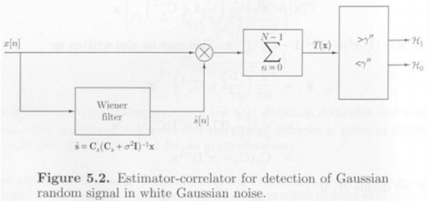
Estimator-Correlator
Example of energy detector
H 0 : x [ n ] = w [ n ] , n = 0 , 1 , ⋯ , N − 1 H 1 : x [ n ] = s [ n ] + w [ n ] , n = 0 , 1 , ⋯ , N − 1 s [ n ] : zero mean, white, WSS Gaussian random process with variance σ s 2 w [ n ] : zero mean WGN with variance σ 2 , independent of the signal \mathcal{H}_0 : x[n] = w[n], \quad n = 0, 1, \cdots, N-1 \\[0.2cm] \mathcal{H}_1 : x[n] = s[n] + w[n], \quad n = 0, 1, \cdots, N-1 \\[0.4cm] s[n] : \text{zero mean, white, WSS Gaussian random process with variance } \sigma_s^2 \\[0.2cm] w[n] : \text{zero mean WGN with variance } \sigma^2, \text{ independent of the signal} H 0 : x [ n ] = w [ n ] , n = 0 , 1 , ⋯ , N − 1 H 1 : x [ n ] = s [ n ] + w [ n ] , n = 0 , 1 , ⋯ , N − 1 s [ n ] : zero mean, white, WSS Gaussian random process with variance σ s 2 w [ n ] : zero mean WGN with variance σ 2 , independent of the signal
NP detector : decide H 1 \mathcal{H}_1 H 1 L ( x ) = p ( x ∣ H 1 ) p ( x ∣ H 0 ) > γ x ∼ { N ( 0 , σ 2 I ) under H 0 N ( 0 , ( σ s 2 + σ 2 ) I ) under H 1 L ( x ) = 1 ( 2 π ( σ s 2 + σ 2 ) ) N / 2 exp [ − 1 2 ( σ s 2 + σ 2 ) ∑ n = 0 N − 1 x 2 [ n ] ] 1 ( 2 π σ 2 ) N / 2 exp [ − 1 2 σ 2 ∑ n = 0 N − 1 x 2 [ n ] ] l ( x ) = N 2 l n ( σ 2 σ s 2 + σ 2 ) + 1 2 ( 1 σ 2 − 1 σ s 2 + σ 2 ) ∑ n = 0 N − 1 x 2 [ n ] l ( x ) = N 2 ln ( σ 2 σ s 2 + σ 2 ) + 1 2 σ s 2 σ 2 ( σ s 2 + σ 2 ) ∑ n = 0 N − 1 x 2 [ n ] → Decide H 1 if T ( x ) = ∑ n = 0 N − 1 x 2 [ n ] > γ ′ : energy detector L(\mathbf{x}) = \frac{p(\mathbf{x}|\mathcal{H}_1)}{p(\mathbf{x}|\mathcal{H}_0)} > \gamma \\[0.4cm] \mathbf{x} \sim \begin{cases} \mathcal{N}(0, \sigma^2 \mathbf{I}) & \text{under } \mathcal{H}_0 \\[0.2cm] \mathcal{N}(0, (\sigma_s^2 + \sigma^2)\mathbf{I}) & \text{under } \mathcal{H}_1 \end{cases}\\[0.2cm] L(\mathbf{x}) = \frac{\frac{1}{(2\pi (\sigma_s^2 + \sigma^2))^{N/2}} \exp\left[-\frac{1}{2(\sigma_s^2 + \sigma^2)} \sum_{n=0}^{N-1} x^2[n] \right]}{\frac{1}{(2\pi \sigma^2)^{N/2}} \exp\left[-\frac{1}{2\sigma^2} \sum_{n=0}^{N-1} x^2[n] \right]} \\[0.4cm]l(\mathbf{x}) = \frac{N}{2} ln\left(\frac{\sigma^2}{\sigma_s^2 + \sigma^2}\right) + \frac{1}{2} \left( \frac{1}{\sigma^2} - \frac{1}{\sigma_s^2 + \sigma^2} \right) \sum_{n=0}^{N-1} x^2[n] \\[0.4cm] l(\mathbf{x}) = \frac{N}{2} \ln\left(\frac{\sigma^2}{\sigma_s^2 + \sigma^2}\right) + \frac{1}{2} \frac{\sigma_s^2}{\sigma^2 (\sigma_s^2 + \sigma^2)} \sum_{n=0}^{N-1} x^2[n] \\[0.4cm]\rightarrow \text{Decide } \mathcal{H}_1 \text{ if } \\[0.4cm] T(\mathbf{x}) = \sum_{n=0}^{N-1} x^2[n] > \gamma' : \text{energy detector} L ( x ) = p ( x ∣ H 0 ) p ( x ∣ H 1 ) > γ x ∼ ⎩ ⎪ ⎨ ⎪ ⎧ N ( 0 , σ 2 I ) N ( 0 , ( σ s 2 + σ 2 ) I ) under H 0 under H 1 L ( x ) = ( 2 π σ 2 ) N / 2 1 exp [ − 2 σ 2 1 ∑ n = 0 N − 1 x 2 [ n ] ] ( 2 π ( σ s 2 + σ 2 ) ) N / 2 1 exp [ − 2 ( σ s 2 + σ 2 ) 1 ∑ n = 0 N − 1 x 2 [ n ] ] l ( x ) = 2 N l n ( σ s 2 + σ 2 σ 2 ) + 2 1 ( σ 2 1 − σ s 2 + σ 2 1 ) n = 0 ∑ N − 1 x 2 [ n ] l ( x ) = 2 N ln ( σ s 2 + σ 2 σ 2 ) + 2 1 σ 2 ( σ s 2 + σ 2 ) σ s 2 n = 0 ∑ N − 1 x 2 [ n ] → Decide H 1 if T ( x ) = n = 0 ∑ N − 1 x 2 [ n ] > γ ′ : energy detector
T ( x ) σ 2 ∼ χ N 2 under H 0 , T ( x ) σ s 2 + σ 2 ∼ χ N 2 under H 1 Q χ ν 2 ( x ) = ∫ x ∞ p ( t ) d t = { 2 Q ( x ) , ν = 1 exp ( − 1 2 x ) ∑ k = 1 ν − 1 2 ( k − 1 ) ! ( 2 x ) k − 1 2 ( 2 k − 1 ) ! , ν > 1 , ν odd exp ( − 1 2 x ) ∑ k = 0 ν 2 − 1 ( x ) k k ! , ν > 1 , ν even P F A = Pr ( T ( x ) > γ ′ ; H 0 ) = Pr ( T ( x ) σ 2 > γ ′ σ 2 ; H 0 ) = Q χ N 2 ( γ ′ σ 2 ) P D = Pr ( T ( x ) > γ ′ ; H 1 ) = Q χ N 2 ( γ ′ σ s 2 + σ 2 ) γ ′ ′ = γ ′ σ 2 ⟹ P D = Q χ N 2 ( γ ′ ′ σ s 2 σ 2 + 1 ) \frac{T(\mathbf{x})}{\sigma^2} \sim \chi^2_N \text{ under } \mathcal{H}_0, \\[0.4cm] \frac{T(\mathbf{x})}{\sigma_s^2 + \sigma^2} \sim \chi^2_N \text{ under } \mathcal{H}_1 \\[0.4cm] Q_{\chi^2_\nu}(x) = \int_x^\infty p(t) dt = \begin{cases} 2Q(\sqrt{x}), & \nu = 1 \\[0.2cm] \exp\left(-\frac{1}{2}x\right)\sum_{k=1}^{\frac{\nu - 1}{2}} \frac{(k-1)! (2x)^{k-\frac{1}{2}}}{(2k-1)!}, & \nu > 1, \nu \text{ odd} \\[0.2cm] \exp\left(-\frac{1}{2}x\right)\sum_{k=0}^{\frac{\nu}{2}-1} \frac{(x)^k}{k!}, & \nu > 1, \nu \text{ even} \end{cases} \\[0.4cm] P_{FA} = \Pr(T(\mathbf{x}) > \gamma' ; \mathcal{H}_0) = \Pr\left(\frac{T(\mathbf{x})}{\sigma^2} > \frac{\gamma'}{\sigma^2}; \mathcal{H}_0\right) = Q_{\chi^2_N}\left(\frac{\gamma'}{\sigma^2}\right) \\[0.4cm] P_D = \Pr(T(\mathbf{x}) > \gamma' ; \mathcal{H}_1) = Q_{\chi^2_N}\left(\frac{\gamma'}{\sigma_s^2 + \sigma^2}\right) \\[0.4cm] \gamma'' = \frac{\gamma'}{\sigma^2} \implies P_D = Q_{\chi^2_N}\left(\frac{\gamma''}{\frac{\sigma_s^2}{\sigma^2} + 1}\right) σ 2 T ( x ) ∼ χ N 2 under H 0 , σ s 2 + σ 2 T ( x ) ∼ χ N 2 under H 1 Q χ ν 2 ( x ) = ∫ x ∞ p ( t ) d t = ⎩ ⎪ ⎪ ⎪ ⎪ ⎪ ⎨ ⎪ ⎪ ⎪ ⎪ ⎪ ⎧ 2 Q ( x ) , exp ( − 2 1 x ) ∑ k = 1 2 ν − 1 ( 2 k − 1 ) ! ( k − 1 ) ! ( 2 x ) k − 2 1 , exp ( − 2 1 x ) ∑ k = 0 2 ν − 1 k ! ( x ) k , ν = 1 ν > 1 , ν odd ν > 1 , ν even P F A = Pr ( T ( x ) > γ ′ ; H 0 ) = Pr ( σ 2 T ( x ) > σ 2 γ ′ ; H 0 ) = Q χ N 2 ( σ 2 γ ′ ) P D = Pr ( T ( x ) > γ ′ ; H 1 ) = Q χ N 2 ( σ s 2 + σ 2 γ ′ ) γ ′ ′ = σ 2 γ ′ ⟹ P D = Q χ N 2 ( σ 2 σ s 2 + 1 γ ′ ′ )
Generalization of energy detector to signals with arbitrary covariance matrixs [ n ] : zero mean, Gaussian random process with covariance matrix C s w [ n ] : zero mean WGN with variance σ 2 , independent of the signal x ∼ { N ( 0 , σ 2 I ) under H 0 N ( 0 , C s + σ 2 I ) under H 1 s[n]: \text{ zero mean, Gaussian random process with covariance matrix } \mathbf{C_s} \\[0.4cm] w[n]: \text{ zero mean WGN with variance } \sigma^2, \text{ independent of the signal} \\[0.4cm] \mathbf{x} \sim \begin{cases} \mathcal{N}(\mathbf{0}, \sigma^2 \mathbf{I}) & \text{under } \mathcal{H}_0 \\[0.2cm] \mathcal{N}(\mathbf{0}, \mathbf{C_s} + \sigma^2 \mathbf{I}) & \text{under } \mathcal{H}_1 \end{cases} s [ n ] : zero mean, Gaussian random process with covariance matrix C s w [ n ] : zero mean WGN with variance σ 2 , independent of the signal x ∼ ⎩ ⎪ ⎨ ⎪ ⎧ N ( 0 , σ 2 I ) N ( 0 , C s + σ 2 I ) under H 0 under H 1
NP detector : decide H 1 \mathcal{H}_1 H 1 L ( x ) = 1 ( 2 π ) N / 2 det ( C s + σ 2 I ) exp ( − 1 2 x T ( C s + σ 2 I ) − 1 x ) 1 ( 2 π ) N / 2 det ( σ 2 I ) exp ( − 1 2 σ 2 x T x ) > γ → − 1 2 x T [ ( C s + σ 2 I ) − 1 − 1 σ 2 I ] x > γ ′ L(\mathbf{x}) = \frac{\frac{1}{(2\pi)^{N/2} \sqrt{\det(\mathbf{C_s} + \sigma^2 \mathbf{I})}} \exp\left(-\frac{1}{2} \mathbf{x}^T (\mathbf{C_s} + \sigma^2 \mathbf{I})^{-1} \mathbf{x}\right)} {\frac{1}{(2\pi)^{N/2} \sqrt{\det(\sigma^2 \mathbf{I})}} \exp\left(-\frac{1}{2 \sigma^2} \mathbf{x}^T \mathbf{x}\right)} > \gamma \\[0.4cm] \rightarrow -\frac{1}{2} \mathbf{x}^T \left[ (\mathbf{C_s} + \sigma^2 \mathbf{I})^{-1} - \frac{1}{\sigma^2} \mathbf{I} \right] \mathbf{x} > \gamma' L ( x ) = ( 2 π ) N / 2 d e t ( σ 2 I ) 1 exp ( − 2 σ 2 1 x T x ) ( 2 π ) N / 2 d e t ( C s + σ 2 I ) 1 exp ( − 2 1 x T ( C s + σ 2 I ) − 1 x ) > γ → − 2 1 x T [ ( C s + σ 2 I ) − 1 − σ 2 1 I ] x > γ ′
T ( x ) = σ 2 x T [ 1 σ 2 I − ( C s + σ 2 I ) − 1 ] x > 2 γ ′ / σ 2 → T ( x ) = x T [ 1 σ 2 ( 1 σ 2 I + C s − 1 ) − 1 ] x T(\mathbf{x}) = \sigma^2 \mathbf{x}^T \left[ \frac{1}{\sigma^2} \mathbf{I} - (\mathbf{C_s} + \sigma^2 \mathbf{I})^{-1} \right] \mathbf{x} > 2 \gamma' / \sigma^2 \\[0.4cm] \rightarrow T(\mathbf{x}) = \mathbf{x}^T \left[ \frac{1}{\sigma^2} \left( \frac{1}{\sigma^2} \mathbf{I} + \mathbf{C_s}^{-1} \right)^{-1} \right] \mathbf{x} T ( x ) = σ 2 x T [ σ 2 1 I − ( C s + σ 2 I ) − 1 ] x > 2 γ ′ / σ 2 → T ( x ) = x T [ σ 2 1 ( σ 2 1 I + C s − 1 ) − 1 ] x
Lets ^ = 1 σ 2 ( 1 σ 2 I + C s − 1 ) − 1 x = 1 σ 2 [ 1 σ 2 C s ( C s + σ 2 I ) C s − 1 ] − 1 x = C s ( C s + σ 2 I ) − 1 x \hat{\mathbf{s}} = \frac{1}{\sigma^2} \left( \frac{1}{\sigma^2} \mathbf{I} + \mathbf{C_s}^{-1} \right)^{-1} \mathbf{x} = \frac{1}{\sigma^2} \left[ \frac{1}{\sigma^2} \mathbf{C_s} (\mathbf{C_s} + \sigma^2 \mathbf{I}) \mathbf{C_s}^{-1} \right]^{-1} \mathbf{x} \\[0.4cm] = \mathbf{C_s} (\mathbf{C_s} + \sigma^2 \mathbf{I})^{-1} \mathbf{x} s ^ = σ 2 1 ( σ 2 1 I + C s − 1 ) − 1 x = σ 2 1 [ σ 2 1 C s ( C s + σ 2 I ) C s − 1 ] − 1 x = C s ( C s + σ 2 I ) − 1 x
Decide H 1 \mathcal{H}_1 H 1 T ( x ) = x T s ^ > γ ′ ′ , T ( x ) = ∑ n = 0 N − 1 x [ n ] s ^ [ n ] T(\mathbf{x}) = \mathbf{x}^T \hat{\mathbf{s}} > \gamma'', \quad T(\mathbf{x}) = \sum_{n=0}^{N-1} x[n] \hat{s}[n] T ( x ) = x T s ^ > γ ′ ′ , T ( x ) = n = 0 ∑ N − 1 x [ n ] s ^ [ n ]
s ^ \hat s s ^ → \rightarrow → MMSE estimator of the signal : Wiener filter estimator
Jointly Gaussian with zero mean → θ ^ = C θ x C x x − 1 x \rightarrow\;\hat \theta=C_{\theta x }C^{-1}_{xx}\text{x} → θ ^ = C θ x C x x − 1 x
Example of energy detector
If the signal is white, C s = σ s 2 I C_s=\sigma^2_sI C s = σ s 2 I s ^ = C s ( C s + σ 2 I ) − 1 x = σ s 2 ( σ s 2 I + σ 2 I ) − 1 x = σ s 2 σ s 2 + σ 2 x \hat{\mathbf{s}} = \mathbf{C}_s (\mathbf{C}_s + \sigma^2 \mathbf{I})^{-1} \mathbf{x} = \sigma_s^2 (\sigma_s^2 \mathbf{I} + \sigma^2 \mathbf{I})^{-1} \mathbf{x} = \frac{\sigma_s^2}{\sigma_s^2 + \sigma^2} \mathbf{x} s ^ = C s ( C s + σ 2 I ) − 1 x = σ s 2 ( σ s 2 I + σ 2 I ) − 1 x = σ s 2 + σ 2 σ s 2 x
→ s ^ [ n ] = σ s 2 σ s 2 + σ 2 x [ n ] \rightarrow \hat{s}[n] = \frac{\sigma_s^2}{\sigma_s^2 + \sigma^2} x[n] → s ^ [ n ] = σ s 2 + σ 2 σ s 2 x [ n ]
Decide H 1 \mathcal{H}_1 H 1 ∑ n = 0 N − 1 x [ n ] s ^ [ n ] = σ s 2 σ s 2 + σ 2 ∑ n = 0 N − 1 x 2 [ n ] > γ ′ ′ \sum_{n=0}^{N-1} x[n] \hat{s}[n] = \frac{\sigma_s^2}{\sigma_s^2 + \sigma^2} \sum_{n=0}^{N-1} x^2[n] > \gamma'' n = 0 ∑ N − 1 x [ n ] s ^ [ n ] = σ s 2 + σ 2 σ s 2 n = 0 ∑ N − 1 x 2 [ n ] > γ ′ ′
∑ n = 0 N − 1 x 2 [ n ] > γ ′ ′ ( σ s 2 + σ 2 ) σ s 2 → energy detector \sum_{n=0}^{N-1} x^2[n] > \frac{\gamma'' (\sigma_s^2 + \sigma^2)}{\sigma_s^2} \quad \rightarrow \text{energy detector} n = 0 ∑ N − 1 x 2 [ n ] > σ s 2 γ ′ ′ ( σ s 2 + σ 2 ) → energy detector N = 2 , C s = σ s 2 [ 1 ρ ρ 1 ] , T ( x ) = x T s ^ = x T C s ( C s + σ 2 I ) − 1 x N = 2, \; C_s = \sigma_s^2 \begin{bmatrix} 1 & \rho \\ \rho & 1 \end{bmatrix}, \; T(x) = x^T \hat{s} = x^T C_s (C_s + \sigma^2 I)^{-1} x N = 2 , C s = σ s 2 [ 1 ρ ρ 1 ] , T ( x ) = x T s ^ = x T C s ( C s + σ 2 I ) − 1 x Let y = V T x , where V = [ 1 2 1 2 1 2 − 1 2 ] : orthogonal matrix, V T = V − 1 \text{Let } y = V^T x, \; \text{where } V = \begin{bmatrix} \frac{1}{\sqrt{2}} & \frac{1}{\sqrt{2}} \\ \frac{1}{\sqrt{2}} & -\frac{1}{\sqrt{2}} \end{bmatrix} : \text{orthogonal matrix, } V^T = V^{-1} Let y = V T x , where V = [ 2 1 2 1 2 1 − 2 1 ] : orthogonal matrix, V T = V − 1 T ( x ) = x T V V T C s V V T x − ( V T x ) T ( V T C s V ) [ V − 1 ( C s + σ 2 I ) ] − 1 ( V T x ) T(x) = x^T VV^T C_s VV^T x - (V^T x)^T (V^T C_s V) [V^{-1} (C_s + \sigma^2 I)]^{-1} (V^T x) T ( x ) = x T V V T C s V V T x − ( V T x ) T ( V T C s V ) [ V − 1 ( C s + σ 2 I ) ] − 1 ( V T x ) = y T Λ s ( Λ s + σ 2 I ) − 1 y = y^T \Lambda_s (\Lambda_s + \sigma^2 I)^{-1} y = y T Λ s ( Λ s + σ 2 I ) − 1 y as V T C s V = Λ s , where Λ s = σ s 2 [ 1 + ρ 0 0 1 − ρ ] \text{as } V^T C_s V = \Lambda_s, \; \text{where } \Lambda_s = \sigma_s^2 \begin{bmatrix} 1 + \rho & 0 \\ 0 & 1 - \rho \end{bmatrix} as V T C s V = Λ s , where Λ s = σ s 2 [ 1 + ρ 0 0 1 − ρ ] → T ( x ) = σ s 2 ( 1 + ρ ) σ s 2 ( 1 + ρ ) + σ 2 y 2 [ 0 ] + σ s 2 ( 1 − ρ ) σ s 2 ( 1 − ρ ) + σ 2 y 2 [ 1 ] \rightarrow T(x) = \frac{\sigma_s^2 (1 + \rho)}{\sigma_s^2 (1 + \rho) + \sigma^2} y^2[0] + \frac{\sigma_s^2 (1 - \rho)}{\sigma_s^2 (1 - \rho) + \sigma^2} y^2[1] → T ( x ) = σ s 2 ( 1 + ρ ) + σ 2 σ s 2 ( 1 + ρ ) y 2 [ 0 ] + σ s 2 ( 1 − ρ ) + σ 2 σ s 2 ( 1 − ρ ) y 2 [ 1 ]
The transformation de-correlates x ( C y \text{x}(C_y x ( C y ) ) )
The energy detector weights the squares of y [ n ] y[n] y [ n ]
V \text{V} V C s C_s C s Λ s \Lambda_s Λ s C s C_s C s Eigen-decomposition : V T C s V = Λ s V^TC_sV=\Lambda_s V T C s V = Λ s V = [ v 0 v 1 ⋯ v N − 1 ] , Λ s = diag ( λ s 0 , λ s 1 , ⋯ , λ s ( N − 1 ) ) , T ( x ) = x T C s ( C s + σ 2 I ) − 1 x = y T Λ s ( Λ s + σ 2 I ) − 1 y = ∑ n = 0 N − 1 λ s n λ s n + σ 2 y 2 [ n ] : canonical form V = \begin{bmatrix} v_0 & v_1 & \cdots & v_{N-1} \end{bmatrix}, \\[0.2cm] \Lambda_s = \text{diag}(\lambda_{s0}, \lambda_{s1}, \cdots, \lambda_{s(N-1)}), \\[0.2cm] T(x) = x^T C_s (C_s + \sigma^2 I)^{-1} x \\[0.2cm] = y^T \Lambda_s (\Lambda_s + \sigma^2 I)^{-1} y \\[0.2cm] = \sum_{n=0}^{N-1} \frac{\lambda_{sn}}{\lambda_{sn} + \sigma^2} y^2[n] \quad : \text{canonical form} V = [ v 0 v 1 ⋯ v N − 1 ] , Λ s = diag ( λ s 0 , λ s 1 , ⋯ , λ s ( N − 1 ) ) , T ( x ) = x T C s ( C s + σ 2 I ) − 1 x = y T Λ s ( Λ s + σ 2 I ) − 1 y = n = 0 ∑ N − 1 λ s n + σ 2 λ s n y 2 [ n ] : canonical form
The weights λ s n λ s n + σ 2 \frac{\lambda_{s_n}}{\lambda_{s_n}+\sigma^2} λ s n + σ 2 λ s n Wiener filter weights in a transformed space
if ρ ≈ 1 \rho\approx1 ρ ≈ 1 σ s 2 > > σ 2 \sigma^2_s>>\sigma^2 σ s 2 > > σ 2 λ s 0 λ s 0 + σ 2 = σ s 2 ( 1 + ρ ) σ s 2 ( 1 + ρ ) + σ 2 ≈ 1 , λ s 1 λ s 1 + σ 2 = σ s 2 ( 1 − ρ ) σ s 2 ( 1 − ρ ) + σ 2 ≈ 0 , v 0 = [ 1 / 2 1 / 2 ] , v 1 = [ 1 / 2 − 1 / 2 ] \frac{\lambda_{s0}}{\lambda_{s0} + \sigma^2} = \frac{\sigma_s^2 (1 + \rho)}{\sigma_s^2 (1 + \rho) + \sigma^2} \approx 1, \\[0.2cm] \frac{\lambda_{s1}}{\lambda_{s1} + \sigma^2} = \frac{\sigma_s^2 (1 - \rho)}{\sigma_s^2 (1 - \rho) + \sigma^2} \approx 0, \\[0.2cm] v_0 = \begin{bmatrix} 1 / \sqrt{2} \\ 1 / \sqrt{2} \end{bmatrix}, \quad v_1 = \begin{bmatrix} 1 / \sqrt{2} \\ -1 / \sqrt{2} \end{bmatrix} λ s 0 + σ 2 λ s 0 = σ s 2 ( 1 + ρ ) + σ 2 σ s 2 ( 1 + ρ ) ≈ 1 , λ s 1 + σ 2 λ s 1 = σ s 2 ( 1 − ρ ) + σ 2 σ s 2 ( 1 − ρ ) ≈ 0 , v 0 = [ 1 / 2 1 / 2 ] , v 1 = [ 1 / 2 − 1 / 2 ]
The component of x \text{x} x v 0 \text{v}_0 v 0 v 1 \text{v}_1 v 1
SNRs for y [ 0 ] y[0] y [ 0 ] y [ 1 ] y[1] y [ 1 ] η 0 2 = E ( y s 2 [ 0 ] ) E ( y w 2 [ 0 ] ) = λ s 0 σ 2 = σ s 2 ( 1 + ρ ) σ 2 ≈ 2 σ s 2 σ 2 ≫ 1 , η 1 2 = E ( y s 2 [ 1 ] ) E ( y w 2 [ 1 ] ) = λ s 1 σ 2 = σ s 2 ( 1 − ρ ) σ 2 ≈ 0 \eta_0^2 = \frac{\mathbb{E}(y_s^2[0])}{\mathbb{E}(y_w^2[0])} = \frac{\lambda_{s0}}{\sigma^2} = \frac{\sigma_s^2 (1 + \rho)}{\sigma^2} \approx \frac{2 \sigma_s^2}{\sigma^2} \gg 1, \\[0.2cm] \eta_1^2 = \frac{\mathbb{E}(y_s^2[1])}{\mathbb{E}(y_w^2[1])} = \frac{\lambda_{s1}}{\sigma^2} = \frac{\sigma_s^2 (1 - \rho)}{\sigma^2} \approx 0 η 0 2 = E ( y w 2 [ 0 ] ) E ( y s 2 [ 0 ] ) = σ 2 λ s 0 = σ 2 σ s 2 ( 1 + ρ ) ≈ σ 2 2 σ s 2 ≫ 1 , η 1 2 = E ( y w 2 [ 1 ] ) E ( y s 2 [ 1 ] ) = σ 2 λ s 1 = σ 2 σ s 2 ( 1 − ρ ) ≈ 0
Linear Model
x = H θ + w θ ∼ N ( 0 , C θ ) , w ∼ N ( 0 , σ 2 I ) H 0 : x = w , H 1 : x = H θ + w s = H θ ∼ N ( 0 , H C θ H T ) Estimator-correlator: decide H 1 if T ( x ) = x T C s ( C s + σ 2 I ) − 1 x > γ ′ ′ → T ( x ) = x T H C θ H T ( H C θ H T + σ 2 I ) − 1 x > γ ′ ′ → equivalent to T ( x ) = x T s ^ = x T H θ ^ where θ ^ is the MMSE estimator of θ ( θ ^ = C θ x C x x − 1 x ) \mathbf{x} = \mathbf{H} \boldsymbol{\theta} + \mathbf{w} \\[0.2cm] \boldsymbol{\theta} \sim \mathcal{N}(\mathbf{0}, \mathbf{C}_{\theta}), \quad \mathbf{w} \sim \mathcal{N}(\mathbf{0}, \sigma^2 \mathbf{I}) \\[0.2cm] \mathcal{H}_0 : \mathbf{x} = \mathbf{w}, \quad \mathcal{H}_1 : \mathbf{x} = \mathbf{H} \boldsymbol{\theta} + \mathbf{w} \\[0.2cm] \mathbf{s} = \mathbf{H} \boldsymbol{\theta} \sim \mathcal{N}(\mathbf{0}, \mathbf{H} \mathbf{C}_{\theta} \mathbf{H}^T) \\[0.2cm] \text{Estimator-correlator: decide } \mathcal{H}_1 \text{ if} \\[0.2cm] T(\mathbf{x}) = \mathbf{x}^T \mathbf{C}_s (\mathbf{C}_s + \sigma^2 \mathbf{I})^{-1} \mathbf{x} > \gamma'' \\[0.2cm] \rightarrow T(\mathbf{x}) = \mathbf{x}^T \mathbf{H} \mathbf{C}_{\theta} \mathbf{H}^T (\mathbf{H} \mathbf{C}_{\theta} \mathbf{H}^T + \sigma^2 \mathbf{I})^{-1} \mathbf{x} > \gamma'' \\[0.2cm] \rightarrow \text{equivalent to } T(\mathbf{x}) = \mathbf{x}^T \hat{\mathbf{s}} = \mathbf{x}^T \mathbf{H} \hat{\boldsymbol{\theta}} \\[0.2cm] \text{where } \hat{\boldsymbol{\theta}} \text{ is the MMSE estimator of } \boldsymbol{\theta} \, (\hat{\boldsymbol{\theta}} = \mathbf{C}_{\theta \mathbf{x}} \mathbf{C}_{\mathbf{xx}}^{-1} \mathbf{x}) x = H θ + w θ ∼ N ( 0 , C θ ) , w ∼ N ( 0 , σ 2 I ) H 0 : x = w , H 1 : x = H θ + w s = H θ ∼ N ( 0 , H C θ H T ) Estimator-correlator: decide H 1 if T ( x ) = x T C s ( C s + σ 2 I ) − 1 x > γ ′ ′ → T ( x ) = x T H C θ H T ( H C θ H T + σ 2 I ) − 1 x > γ ′ ′ → equivalent to T ( x ) = x T s ^ = x T H θ ^ where θ ^ is the MMSE estimator of θ ( θ ^ = C θ x C x x − 1 x ) General Gaussian Detection
Detection of a signal which is composed of a deterministic component and a random componentH 0 : x = w , H 1 : x = s + w w ∼ N ( 0 , C w ) , s ∼ N ( μ s , C s ) : deterministic component becomes the mean. \mathcal{H}_0 : \mathbf{x} = \mathbf{w}, \quad \mathcal{H}_1 : \mathbf{x} = \mathbf{s} + \mathbf{w} \\[0.2cm] \mathbf{w} \sim \mathcal{N}(\mathbf{0}, \mathbf{C}_w), \quad \mathbf{s} \sim \mathcal{N}(\boldsymbol{\mu}_s, \mathbf{C}_s) : \text{deterministic component becomes the mean.} H 0 : x = w , H 1 : x = s + w w ∼ N ( 0 , C w ) , s ∼ N ( μ s , C s ) : deterministic component becomes the mean.
Decide H 1 \mathcal{H}_1 H 1 p ( x ∣ H 1 ) p ( x ∣ H 0 ) = 1 ( 2 π ) N / 2 det ( C s + C w ) exp ( − 1 2 ( x − μ s ) T ( C s + C w ) − 1 ( x − μ s ) ) 1 ( 2 π ) N / 2 det ( C w ) exp ( − 1 2 x T C w − 1 x ) > γ T ( x ) = x T C w − 1 x − ( x − μ s ) T ( C s + C w ) − 1 ( x − μ s ) = x T C w − 1 x − x T ( C s + C w ) − 1 x + 2 x T ( C s + C w ) − 1 μ s − μ s T ( C s + C w ) − 1 μ s \frac{p(\mathbf{x}|\mathcal{H}_1)}{p(\mathbf{x}|\mathcal{H}_0)} = \frac{ \frac{1}{(2\pi)^{N/2} \sqrt{\det(\mathbf{C}_s + \mathbf{C}_w)}} \exp\left(-\frac{1}{2} (\mathbf{x} - \boldsymbol{\mu}_s)^T (\mathbf{C}_s + \mathbf{C}_w)^{-1} (\mathbf{x} - \boldsymbol{\mu}_s) \right) }{ \frac{1}{(2\pi)^{N/2} \sqrt{\det(\mathbf{C}_w)}} \exp\left(-\frac{1}{2} \mathbf{x}^T \mathbf{C}_w^{-1} \mathbf{x} \right) } > \gamma \\[0.2cm] T(\mathbf{x}) = \mathbf{x}^T \mathbf{C}_w^{-1} \mathbf{x} - (\mathbf{x} - \boldsymbol{\mu}_s)^T (\mathbf{C}_s + \mathbf{C}_w)^{-1} (\mathbf{x} - \boldsymbol{\mu}_s) \\[0.2cm] = \mathbf{x}^T \mathbf{C}_w^{-1} \mathbf{x} - \mathbf{x}^T (\mathbf{C}_s + \mathbf{C}_w)^{-1} \mathbf{x} + 2 \mathbf{x}^T (\mathbf{C}_s + \mathbf{C}_w)^{-1} \boldsymbol{\mu}_s - \boldsymbol{\mu}_s^T (\mathbf{C}_s + \mathbf{C}_w)^{-1} \boldsymbol{\mu}_s p ( x ∣ H 0 ) p ( x ∣ H 1 ) = ( 2 π ) N / 2 d e t ( C w ) 1 exp ( − 2 1 x T C w − 1 x ) ( 2 π ) N / 2 d e t ( C s + C w ) 1 exp ( − 2 1 ( x − μ s ) T ( C s + C w ) − 1 ( x − μ s ) ) > γ T ( x ) = x T C w − 1 x − ( x − μ s ) T ( C s + C w ) − 1 ( x − μ s ) = x T C w − 1 x − x T ( C s + C w ) − 1 x + 2 x T ( C s + C w ) − 1 μ s − μ s T ( C s + C w ) − 1 μ s
By matrix inversion lemmaC w − 1 − ( C s + C w ) − 1 = C w − 1 C s ( C s + C w ) − 1 , T ′ ( x ) = x T ( C s + C w ) − 1 μ s + 1 2 x T C w − 1 C s ( C s + C w ) − 1 x . \mathbf{C}_w^{-1} - (\mathbf{C}_s + \mathbf{C}_w)^{-1} = \mathbf{C}_w^{-1} \mathbf{C}_s (\mathbf{C}_s + \mathbf{C}_w)^{-1}, \\[0.2cm] T'(\mathbf{x}) = \mathbf{x}^T (\mathbf{C}_s + \mathbf{C}_w)^{-1} \boldsymbol{\mu}_s + \frac{1}{2} \mathbf{x}^T \mathbf{C}_w^{-1} \mathbf{C}_s (\mathbf{C}_s + \mathbf{C}_w)^{-1} \mathbf{x}. C w − 1 − ( C s + C w ) − 1 = C w − 1 C s ( C s + C w ) − 1 , T ′ ( x ) = x T ( C s + C w ) − 1 μ s + 2 1 x T C w − 1 C s ( C s + C w ) − 1 x .
As special cases,
If C s = 0 C_s=0 C s = 0 s = μ s s=\mu_s s = μ s T ′ ( x ) = x T C w − 1 μ s T'(\text{x})=\text{x}^TC^{-1}_{\text{w}}\mu_s T ′ ( x ) = x T C w − 1 μ s
If μ s = 0 \mu_s=0 μ s = 0 s ∼ N ( 0 , C s ) s\sim\mathcal{N}(0,C_s) s ∼ N ( 0 , C s ) T ′ ( x ) = 1 2 x T C w − 1 C s ( C s + C w ) − 1 x = 1 2 x T C w − 1 s ^ T'(\text{x})=\frac{1}{2}\text{x}^TC^{-1}_\text{w}C_s(C_s+C_\text{w})^{-1}\text{x}=\frac{1}{2}\text{x}^TC^{-1}_\text{w}\hat s T ′ ( x ) = 2 1 x T C w − 1 C s ( C s + C w ) − 1 x = 2 1 x T C w − 1 s ^ s ^ = C s ( C s + C w ) − 1 x \hat s=C_s(C_s+C_\text{w})^{-1}\text{x} s ^ = C s ( C s + C w ) − 1 x s s s
All Content has been written based on lecture of Prof. eui-seok.Hwang in GIST(Detection and Estimation)