Review

Cramer-Rao Lower Bound(CRLB)

• The CRLB give a lower bound on the variance of any unbiased estimator

  Does not guarantee bound can be obtained

• If find an unbiased estimator whose variance = CRLB then it's MVUE
• Otherwise can use Ch.5 tools(Rao-Blackwell-Lehmann-Scheffe Theorem and Neyman-Fisher Factorization Theorem) to construct a better estimator from any unbiased one - possibly the MVUE if conditions are met

CRLB -Scalar parameter

• Let $p(x;\theta)$ satisfy the regularity condition,
  $E\left[\frac{\partial \ln p(x;\theta)}{\partial \theta}\right] =0\;\text{for all }\theta$
• Then, the variance of any unbiased estimator $\hat\theta$ must satisfy
  $\text{var}(\hat\theta)\geq\frac{1}{-E\left[\frac{\partial^2\ln p(x;\theta)}{\partial\theta^2}\right]}=\frac{1}{E\left[\left(\frac{\partial\ln p(x;\theta)}{\partial\theta}\right)^2\right]}=\frac{1}{I(\theta)}$
• Where the derivative is evaluated at the true value of $\theta$ and the expectation is taken w.r.t. $p(x;\theta).

  Furthermore, an unbiased estimator may be found that attains the bound for all $\theta$ iff

  $\frac{\partial\ln p(x;\theta)}{\partial\theta}=I(\theta)(g(x)-\theta)$

  For some functions $g(x)$ and $I$. That estimator $\hat\theta =g(x)$, is the MVUE with variance is $I(\theta)$

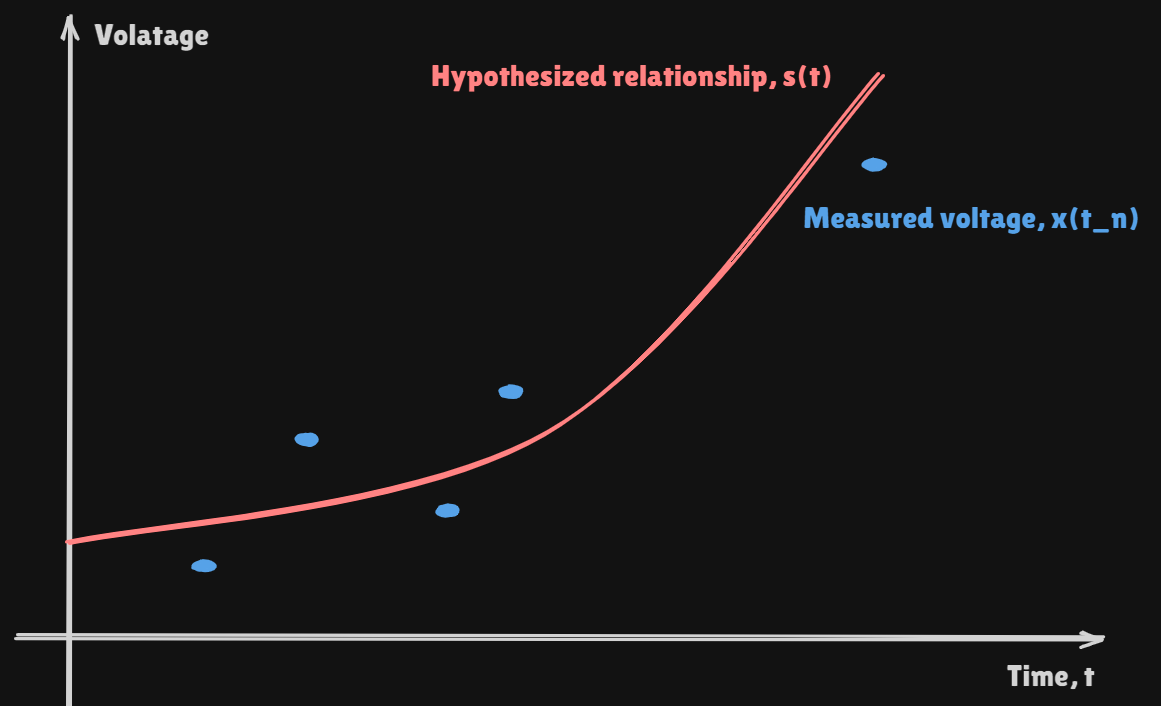
General CRLB for Signals in WGN

Vector Form of the CRLB

• Assuming $p(x;\theta)$ satisfies the regularity condition
  $E\left[\frac{\partial \ln p(x;\theta)}{\partial\theta}\right] =0,\;\text{for all } \theta$
• The covariance matrix of any unbiased estimator $\hat \theta$ satisfies
  $C_{\hat\theta}-I^{-1}(\theta)\geq0\quad[I(\theta)]_{ij}=-E\left[\frac{\partial\ln p(x;\theta)}{\partial\theta_i\partial\theta_j}\right]$
• Where $\geq 0$ means the matrix is positive semidefinite

  Furthermore, an unbiased estimator may be found that attains the bound
  $C_{\hat\theta}=I^{-1}(\theta)$ if and only if

  $\frac{\partial \ln p(x;\theta)}{\partial \theta} = I(\theta)(g(x) - \theta)$
• In that case, $\hat \theta = g(x)$ is the MVU estimator with variance $I^{-1}(\theta)$.

Linear Model 으악

• The determination of the MVUE is difficult in general. Many estimation problems can be represented by the linear model for which the MVUE is easily determined
• Line fitting example
  $x[n]=A+Bn+w[n],\quad n=0,1,\dots,N-1,\;w[n]:\text{WGN}$
  • In Matrix notation,
    $\text{x} =H\theta +w : \text{linear model}\\ \text{x} = \begin{matrix}\left[x[0]\;x[1]\;\cdots x[N-1]\right]\end{matrix}^T,\\ w=[w[0]\;w[1]\;\cdots\;w[N-1]]^T\;w\sim\mathcal{N}(0,\sigma^2I)\\ \theta=[A\;B]^T\\[0.5cm] \mathbf{H} = \begin{bmatrix} 1 & 0 \\ 1 & 1 \\ \vdots & \vdots \\ 1 & N-1 \end{bmatrix}$

MVUE for the Linear Model

• Determine the MVUE from the equality condition of CRLB theorem
• $\hat \theta =g(x)$ will be the MVUE if
  $\frac{\partial \ln p(x;\theta)}{\partial \theta} =I(\theta)(g(x)-\theta)\quad \text{with }C_{\hat\theta}=I^{-1}(\theta)\\ P(\underline{n} ; \underline{\theta}) = \prod_{n=0}^{N-1} P(x(n) ; \underline{\theta})$
• For the linear model,
  $\frac{\partial \ln p(x;\theta)}{\partial\theta}=\frac{\partial}{\partial\theta}\left[-\ln(2\pi\sigma^2)^{\frac{N}{2}}-\frac{1}{2\sigma^2}(\text{x}-\text{H}\theta)^T(\text{x}-\text{H}\theta)\right]\\ =-\frac{1}{2\sigma^2}\frac{\partial}{\partial\theta}[\text{x}^T\text{x}-2\text{x}^T\text{H}\theta +\theta^T\text{H}^T\text{H}\theta]\\ =\frac{1}{\sigma^2}[\text{H}^2\text{x}-\text{H}^T\text{H}\theta]$
• Assume that $\text{H}^T\text{H}$ is invertible
  $\frac{\partial\ln p(x;\theta)}{\partial\theta}=\frac{\text{H}^T\text{H}}{\sigma^2}[(\text{H}^T\text{H})^{-1}\text{H}^T\text{x}-\theta]\approx I(\theta)(g(x)-\theta)\\ \rightarrow\hat\theta=(\text{H}^T\text{H})^{-1}\text{H}^T\text{x},\quad I(\theta)=\frac{\text{H}^T\text{H}}{\sigma^2}\\ C_{\hat\theta}=I^{-1}(\theta)=\sigma^2(\text{H}^T\text{H})^{-1}$
• For linear model, an efficient MVUE can be found if $\text{H}^T\text{H}$ is invertible. $\text{H}^T\text{H}$ is invertible iff(if and only iff) the columns of $\text{H}$ are linearly independent.(see Prob. 4.2)
• If the columns of $\text{H}$ are not linearly independent, even in the absence of noise, the model parameters will not be identificable(The number of equations is less than the number of variables.)

MVUE for the Linear Model - Theorem

• If the observed data can be modeled as $\text{x}=\text{H}\theta+\text{w}$, then the MVUE is
  $\hat \theta=(\text{H}^T\text{H})^{-1}\text{H}^T\text{x}$
• And the covariance matrix of $\hat\theta$ is
  $C_{\hat\theta}=I^{-1}(\theta)=\sigma^2(\text{H}^T\text{H})^{-1}$
• Where $\text{x}$ is an $N\times 1$ vector of observations, $\text{H}$ is known $N\times p$ observation matrix(with $N > p$) with rank $p$
• $\theta$ is a $p\times 1$ vector of parameters to be estimated, and $\text{w}$ is an $N\times 1$ noise vector with PDF $\mathcal{N}(0, \sigma^2I)$
• For the linear model the MVUE is efficient in that it attains the CRLB.
• Also, the statistical performance of $\hat\theta$ is completely specified, because $\hat\theta$ is a linear transformation of a Gaussian vecot $\text{x}$ and hence
  $\hat\theta\sim\mathcal{N}(\theta, \sigma^2(\text{H}^T\text{H})^{-1})$

Example - Curve Fitting

The Linear in Linear Model does not come from fitting straight lines to data. It is more general than that!!

Example - Fourier Analysis

• Data model
  $x[n]=\displaystyle\sum_{k=1}^Ma_k \cos\left(\frac{2\pi kn}{N}\right)+\displaystyle\sum_{k=1}^Mb_k\sin\left(\frac{2\pi kn}{N}\right) + w[n],\quad n=0,1,\cdots,N-1$
• Parameters(Fourier coefficients)
  $\theta=[a_1\;a_2\;\cdots\;a_M\;b_1\;b_2\;\cdots\;b_M]^T$
• Observation matrix
  $\mathbf{H} = \begin{bmatrix} 1 & \cdots & 1 & 0 & \cdots & 0 \\ \cos\left(\frac{2\pi}{N}\right) & \cdots & \cos\left(\frac{2\pi M}{N}\right) & \sin\left(\frac{2\pi}{N}\right) & \cdots & \sin\left(\frac{2\pi M}{N}\right) \\ \vdots & \cdots & \vdots & \vdots & \cdots & \vdots \\ \cos\left(\frac{2\pi (N-1)}{N}\right) & \cdots & \cos\left(\frac{2\pi M (N-1)}{N}\right) & \sin\left(\frac{2\pi (N-1)}{N}\right) & \cdots & \sin\left(\frac{2\pi M (N-1)}{N}\right) \\ \end{bmatrix}\\ = [\mathbf{h}_1 \ \mathbf{h}_2 \ \cdots \ \mathbf{h}_{2M}] \quad \rightarrow \quad \mathbf{h}_i^T \mathbf{h}_j = 0 \ \text{for} \ i \neq j$
• Apply MVUE Theorem for Linear Model, $\hat\theta=(\text{H}^T\text{H})^{-1}\text{H}^T\text{x}$
  $\mathbf{H}^T \mathbf{H} = \begin{bmatrix} \mathbf{h}_1^T \\ \vdots \\ \mathbf{h}_{2M}^T \end{bmatrix} [\mathbf{h}_1 \ \mathbf{h}_2 \ \cdots \ \mathbf{h}_{2M}] = \begin{bmatrix} N/2 & 0 & \cdots & 0 \\ 0 & N/2 & \cdots & 0 \\ \vdots & \vdots & \ddots & \vdots \\ 0 & 0 & \cdots & N/2 \end{bmatrix} = \frac{N}{2} \mathbf{I}\\ \hat{\theta} = \frac{2}{N} \mathbf{H}^T \mathbf{x} = \begin{bmatrix} \frac{2}{N} \mathbf{h}_1^T \mathbf{x} \\ \vdots \\ \frac{2}{N} \mathbf{h}_{2M}^T \mathbf{x} \end{bmatrix} \rightarrow \begin{cases} \hat{a}_k = \frac{2}{N} \sum_{n=0}^{N-1} x[n] \cos\left( \frac{2\pi kn}{N} \right) \\ \hat{b}_k = \frac{2}{N} \sum_{n=0}^{N-1} x[n] \sin\left( \frac{2\pi kn}{N} \right) \end{cases}\\ \rightarrow E(\hat{a}_k) = a_k, \ E(\hat{b}_k) = b_k, \ \mathbf{C}_{\hat{\theta}} = \sigma^2 (\mathbf{H}^T \mathbf{H})^{-1} = \frac{2\sigma^2}{N} \mathbf{I}$

Example - System Identification

• Goal : Determine a model for the system

  • Wireless Communications(idenfy & equalize multi-path)
  • Geophysical Sensing(oil exploration)
  • Speakerphone(echo cancellation)

• In many applications : assume that the system is FIR(Finite Impulse Response)(length p)(or TDL)

  $x[n] =\displaystyle\sum_{k=0}^{p-1}h[k]u[n-j]+w[n],\quad n=0,\cdots,N-1$

• where $u[n]$: Pilot Signal is known, $u[n] =0$ for $n < 0$, $w[n]$: WGN

  $\mathbf{x} = \begin{bmatrix} u[0] & 0 & \cdots & 0 \\ u[1] & u[0] & \cdots & 0 \\ \vdots & \vdots & \ddots & \vdots \\ u[N-1] & u[N-2] & \cdots & u[N-p] \end{bmatrix} \begin{bmatrix} h[0] \\ h[1] \\ \vdots \\ h[p-1] \end{bmatrix} + \mathbf{w} = \underline\mathbf{H}\underline\theta + \underline\mathbf{w}$

  It's Linear than, We can apply MVUE

• MVU estimator of the impulse response

  $\hat \theta=(\text{H}^T\text{H})^{-1}\text{H}^T\text{x},\quad C_{\hat\theta}=\sigma^2(\text{H}^T\text{H})^{-1}$

  What signal $u[n]$ is best to use?

• The $u[n]$ that gives the smallest estimated variances!!

• Choosing $u[n]$ s.t. $\text{H}^T\text{H}$ is diagonal will minimize variance

• Choose $u[n]$ to be pseudo-random noise(PRN)

  • $\rightarrow u[n] \text{ is } \perp \text{ to all its shifts } u[n - m]$

    PRN has approximately flat spectrum(From a frequency-domain view a PRN signal equally probes at all frequencies)

• Designing the probing signal

  $\text{var}(\hat\theta_i)=\text{e}^T_iC_{\hat\theta}\text{e}_i,\quad \text{e}_i=[0\;0\;\cdots\;0\;1\;0\;\cdots\;0]^T:\text{one hot vector},\;C^{-1}_{\hat\theta}=\text{D}^T\text{D}\\ 1^2 = \left( \mathbf{e}_i^T \mathbf{D}^T \mathbf{D} \mathbf{D}^{T^{-1}} \mathbf{e}_i \right)^2, \text{ let } \boldsymbol{\xi}_1 = \mathbf{D} \mathbf{e}_i, \ \boldsymbol{\xi}_2 = \mathbf{D}^{T^{-1}} \mathbf{e}_i, \text{ then } 1 = \left( \boldsymbol{\xi}_1^T \boldsymbol{\xi}_2 \right)^2\\ \rightarrow \text{var}(\hat\theta_i)\geq\frac{1}{\text{e}^T_iC^{-1}_{\hat\theta}\text{e}_i}=\frac{\sigma^2}{[\text{H}^T\text{H}}]_{ii}$

• Equality holds when $\xi_1=c\xi_2$ or $\mathbf{D} \mathbf{e}_i = c_i \mathbf{D}^{T^{-1}} \mathbf{e}_i, \ i = 1, 2, \dots, p.$

  $\rightarrow \mathbf{D}^T \mathbf{D} \mathbf{e}_i = c_i \mathbf{e}_i \quad \rightarrow \frac{\mathbf{H}^T \mathbf{H}}{\sigma^2} \mathbf{e}_i = c_i \mathbf{e}_i, \quad i = 1, 2, \dots, p$

• The conditions achieving the minimum possible variances are

  $\mathbf{H}^T \mathbf{H} = \sigma^2 \begin{bmatrix} c_1 & 0 & \cdots & 0 \\ 0 & c_2 & \cdots & 0 \\ \vdots & \vdots & \ddots & \vdots \\ 0 & 0 & \cdots & c_p \end{bmatrix}$

• To minimize the variance of MVUE, $u[n]$ should be chosen to make $\text{H}^T\text{H}$ diagonal

  $[\mathbf{H}^T \mathbf{H}]_{ij} = \sum_{n=1}^{N} u[n - i] u[n - j], \quad i = 1, \dots, p, \quad j = 1, \dots, p$

  For large $N$, we have

  $[\mathbf{H}^T \mathbf{H}]_{ij} \approx \sum_{n=0}^{N-1-|i-j|} u[n] u[n + |i - j|] \quad (\text{correlation function of } u[n])\\ \mathbf{H}^T \mathbf{H} = N \begin{bmatrix} r_{uu}[0] & r_{uu}[1] & \cdots & r_{uu}[p-1] \\ r_{uu}[1] & r_{uu}[0] & \cdots & r_{uu}[p-2] \\ \vdots & \vdots & \ddots & \vdots \\ r_{uu}[p-1] & r_{uu}[p-2] & \cdots & r_{uu}[0] \end{bmatrix} \quad : \text{Toeplitz matrix}\\[0.3cm] r_{uu}[k] = \frac{1}{N} \sum_{n=0}^{N-1-k} u[n] u[n+k]\\ \rightarrow \text{To make it diagonal, }\\ r_{uu}[k] = 0 \text{ for } k \neq 0 \rightarrow \text{Pseudorandom noise (PRN)}$

• Under these conditions, $\text{H}^T\text{H}=Nr_{uu}[0]I$

  $\rightarrow \text{var}(\hat{h}[i]) = \frac{\sigma^2}{N r_{uu}[0]}, \quad i = 0, 1, \dots, p-1$

• Then, MVU estimator $\hat\theta = (\text{H}^T\text{H})^{-1}\text{H}^T\text{x}$ with $\text{H}^T\text{H}=Nr_{uu}[0]I$ yields

  $\hat{h}[i] = \frac{1}{N r_{uu}[0]} \sum_{n=0}^{N-1} u[n-i] x[n]\\ = \frac{1}{N} \sum_{n=0}^{N-1-i} \frac{u[n] x[n+i]}{r_{uu}[0]}\\ = \frac{r_{ux}[i]}{r_{uu}[0]}, \quad i = 0, 1, \dots, p-1$

  wiener filter : has been cross corelations and autocorelations function so far about WGN

Linear Model with Colored Noise

• General Linear Model with colored noise
  $\text{w}\sim\mathcal{N}(0,C)$

  Whitening approach

  $\mathbf{C}^{-1} = \mathbf{D}^T \mathbf{D}, \quad \mathbf{D} : \text{invertible } N \times N \text{ matrix: whitening transformation} \\ E[(\mathbf{D}\mathbf{w})(\mathbf{D}\mathbf{w})^T] = \mathbf{DCD}^T = \mathbf{DD}^{-1} \mathbf{D}^T \mathbf{D}^T = \mathbf{I} \\ \text{Transform to whitened model:} \quad \mathbf{x} = \mathbf{H}\boldsymbol{\theta} + \mathbf{w} \quad \rightarrow \quad \mathbf{x}' = \mathbf{D} \mathbf{x} = \mathbf{D} \mathbf{H} \boldsymbol{\theta} + \mathbf{D} \mathbf{w} = \mathbf{H}' \boldsymbol{\theta} + \mathbf{w}' \\ \mathbf{w}' \sim \mathcal{N}(0, \mathbf{I}) \\ \hat{\boldsymbol{\theta}} = (\mathbf{H}'^T \mathbf{H}')^{-1} \mathbf{H}'^T \mathbf{x}' = (\mathbf{H}^T \mathbf{D}^T \mathbf{D} \mathbf{H})^{-1} \mathbf{H}^T \mathbf{D}^T \mathbf{D} \mathbf{x} = (\mathbf{H}^T \mathbf{C}^{-1} \mathbf{H})^{-1} \mathbf{H}^T \mathbf{C}^{-1} \mathbf{x} \\ \mathbf{C}_{\hat{\boldsymbol{\theta}}} = (\mathbf{H}'^T \mathbf{H}')^{-1} = (\mathbf{H}^T \mathbf{C}^{-1} \mathbf{H})^{-1}$

All Content has been written based on lecture of Prof. eui-seok.Hwang in GIST(Detection and Estimation)