Recap
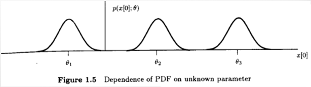
Revisit : Likelihood Function
- The
Likelihood Function(same description of PDF) - But as a function of parameter w/ the data vector fixed
 |  |
|---|
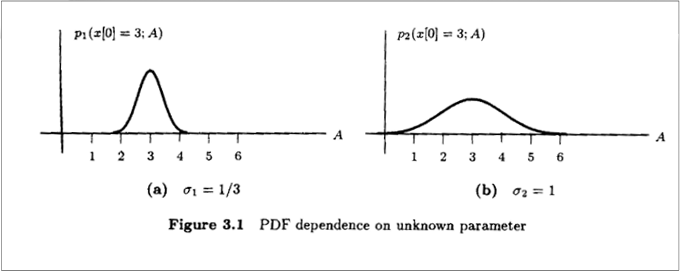
Likelihood Function Characteristics
- Intuitively :
sharpnessof theLikelihood Functionsets accuracy Sharpnessis measured usingcurvature:- Curvature ↑ ⇒ PDF concentration ↑ ⇒ Accuracy ↑
- Expected sharpness of
likelihood function
Vector Form of the CRLB
- Assuming satisfies the
regularity condition - The
covariance matrixof anyunbiased estimatorsatisfieswhere means the matrix ispositive semidefinite - Furthermore, an
unbiased estimatormay be found that attains the bound
if and only if - In that case, is the
MVUEwithvariance
MVUE for the Linear Model - Theorem
- If the observed data can be modeled as ,
- The
MVUEis - And the
covariance matrixof is - For the
linear model, theMVUEisefficientin that attains theCRLB - Also, the statiscal performance of is completely specified, because is a
linear transformationof aGaussian vectorand hence
Finding the MVUE so far
- When the observations and the data are related in a
linear way, - and the noise was
Gaussian, then theMVUEwas easy to find:withcovariance matrix, - Using the
CRLB, if you got lucky, then you could writewhere would be yourMVUE, anefficient estimator(meet theCRLB) - Even if
no efficient estimatorexists, anMVUEmay exist - In this section, we try to find a systematic way of determining the
MVUEif it exists
Finding the MVUE
- We wish to estimate the parameter(s) from the observations
- Step 1
- Determine (if possible) a
sufficient statisticfor the parameter to be estimated - This may be done using the
Neyman-Fisher factorization theorem
- Determine (if possible) a
- Step 2
- Determine whether the
sufficient statisticis alsocompleteThis is generally hard to do
- If it is
not complete, we can say nothing more about theMVUE - If it is, continue to
Step 3
- Determine whether the
- Step 3
- Find the
MVUEfrom is one of two ways using the
Rao-Blackwell-Lehmann-Scheffe(RBLS) theoremRao-Blackwell-Lehmann_Scheffe(RBLS) theorem
- Find a function of the
sufficient statisticthat yields anunbiasedestimator , theMVUE - By definition of
completenessof the statistic, this will yield theMVUE - Find any
unbiasedestimator for , and then determine
- This is usually very tedious/difficult to do
- The expectation is taken over the distribution
- Find a function of the
- Find the
- Step 1
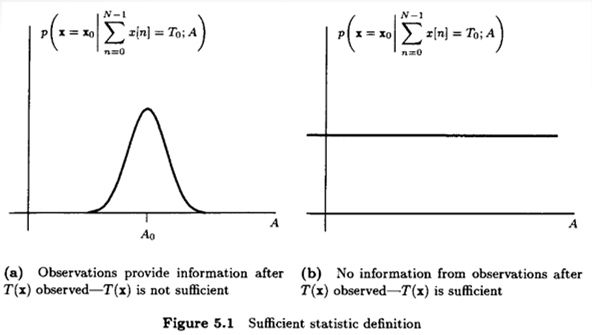
Sufficient Statistics
- Example : Estimating a DC Level in WGN
- :
MVUEwithvariance - :
unbiasedestimator withvariance
disarded the data points which carryinformationabout
- :
- Is there a set of data that is
sufficient?- :
sufficient statistic
(Original data set is alwayssufficient) - :
sufficient statistic - :
minimalsufficient statistis (least # of elements)
- :
- For estimation of , once we know , we
no longer needthe individualdatavaluesSince
all informationhas been summarized in thesufficient statistic - A statistic is the result of applying a function to a set of data - our observations
- A
single statisticis asingle functionof the observations, - And it is called
sufficient statisticsif the PDF isindependentof
- Example : Estimating a DC Level in WGN
- Conditional PDF should
not dependon
- Verification of a
sufficient statisticThen,Independentof the parameter
→ issufficient statisticfor the estimation of
- Evaluation of the
conditional PDFis difficult Guessinga potentialsufficient statisticsis even more difficult- General framework to find
sufficient statistic:Neyman-Fisher facorization
Neyman-Fisher Factorization
- If we can factor the PDF aswhere is a function depending on only through and is a function
dependingonly on - Then is a
sufficient statisticfor - Conversely, if is a
sufficient statisticfor , then the PDF can be factored as in the above equation - Proof : Appendix 5A
Example 1
- Example : Estimating a DC Level in WGN
- Note that any one-to-one function of is a
sufficient statistic
Example 2
- Example : Power of WGN
is theunknown parameter
Naturally Extended Neyman-Fisher Factorization
- The statistics are
joint sufficient statistics
if the conditional pdf does not depend on - They are
joint sufficient statisticsif and only if the pdf may be factored as - The original data are always
sufficient statistics
Phase Examples
- The exponent may be expanded as
- No single
sufficient statisticexists, butjointly sufficient statisticsexist
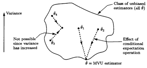
Sufficient Statistics and MVUEs
-
If we determined a
sufficient statisticfor -
Then we can use this to improve any
unbiased estimatorof -
As is proven in the
Rao-Blackwell-Lehmann-Scheffe(RBLS) theorem -
If we're lucky and the statistic is also
complete, we can use it to find theMVUE- There are many definitions for the
completenessof a statistic
One that is easy for us to use in the context of estimation is the following :It is called
completeif only 1 function of it yields anunbiased estimatorof
- This is generally difficult to check but is easy conceptually
- Another way of checking if a statistic is
complete:
- A statistic is
completeit contains above for all is only
satisfied by for all
- There are many definitions for the
Example : DC Level in WGN
- Suppose we don't know that the sample mean is
MVUE, but know thatis asufficient statistic - Two ways to find the
MVUE:- Find any
unbiased estimatorof , say , and determine
The expectation is taken with respect to - Find some function so that is an
unbiasedestimator of
- Find any
First Approach to find
- For
jointly Gaussian random variablesand(Appendix 10A)
Second Approach
- For
unbiased
Rao-Blackwell-Lehmann-Scheffe(RBLS) Theorem
- If is an
unbiased estimatorof and is asufficient statisticfor ,
Then- A valid estimator for (not dependent on )
Unbiased- Of lesser or equal variance thant that of , for all
- Additionally, if the
sufficient statisticiscomplete, then is theMVUE - A statistic is
completeif there is only one function of the statistic that isunbiased - doesn't depend on by the definition of
sufficient statistic
1is proven - Note that since
- Thus, :
3is proven
- If is
complete, there is only one function of that is anunbiasedestimator- is unique independent of
- for all
- must be an
MVUE
Completenessdepends on the PDF of- This condition is satisfied for the exponential family of PDFs
RBLS Example
Incomplete sufficient statistic- is
sufficient statisticand anunbiased estimatorIs a
MVUE?- Suppose that there exists another function w/ the
unbiasedproperty
and see if - Let , then for all
- Since for all
- satisfies the condition
⇒ based on thesufficient statisticand isunbiased→No
- Suppose that there exists another function w/ the
- Completeness condition is that only the zero function satisfies
Procedure for finding
MVUE(Scalar)- Use
Neyman-Fisher Factorizationto findsufficient statistic - Determine if is
complete;
The condition forcompletenessis that only the zero function
satisfies for all - Find a function of that is
unbiased
Then is theMVUE
Or alternatively, evaluate where is anyunbiased estimator
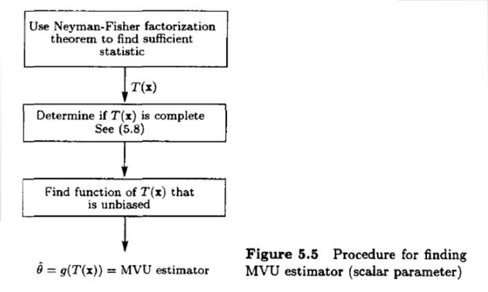
- Use
Example : Mean of Uniform Noise
- Consider estimating the mean of the i.i.d. uniform noise
- Find an
efficient estimator- The
regularity conditiondoes not hold :CRLBcannot be applied - Natural guess : sample mean estimator
- Is the sample mean estimator
MVUE?
- The
- Follow Figure 5.5 unit step function
- :
sufficient statisticfor , and alsocomplete - Next, we need to find a function of that is
unbiased - To make this
unbiasedThe sample mean estimator was not theMVUE - Smaller than the variance of sample mean estimator for
- Not easy to apply when there is no single
sufficient statistic
Extensions to Vector Parameters
- If we can factor the PDF as
- is a function
depending ononly through , an statistic - And is function
depending on - Then is a
sufficient statisticfor - Conversely, if is a
sufficient statisticfor , then the PDF can be factored as above - Sufficiency : is
sufficientfor the estimation of if
RBLS
- If is an
unbiasedestimator of and is ansufficientstatistic for
Then is- A valid estimator for ( not dependent on )
Unbiased- Of lesser or equal variance than that of (each element of has less or equal variance)
- Additionally, if the
sufficient statisticiscomplete
then is theMVUECompleteness: if for , an arbitrary function of- for all , then for all

AI, Security