Introduction

• Up to now - Classical Approach : the parameter is a deterministic but unknown constant
  • Assumes $\theta$ is deterministic
  • Variance of the estimate could depend on $\theta$
  • In Monte Carlo simulations:
    • $M$ runs done at the same $\theta$, must do $M$ runs at each $\theta$ of interest
    • Averaging done over data, No averaging over $\theta$ values

---

• From now on - Bayesian Approach : the parameter is a random variable whose particular realization we must estimate
  • Assumes $\theta$ is random with pdf $p(\theta)$
  • Variance of the estimate CAN'T depend on $\theta$
  • In Monte Carlo simulations
    • Each run done at a randomly chosen $\theta$
    • Averaging done over data AND over $\theta$ values

Motivation

• Sometimes we have prior knowledge on $\theta \rightarrow$ some values are more likely than others
• Useful when the classical MVUE does not exist because of non-uniformity of minimal variance → optimal on the average
  
  To combat the signal estimation problem estimate signal $\text{s}$
  $\text{x}=\text{s}+\text{w}$
  • Classical solution : $\hat\text{s}=(\text{I}^T\text{I})^{-1}\text{I}^T\text{x}=\text{x}$
  • Bayesian solution : the Wiener filter

Prior Knowledge and Estimation

• The use of prior knowledge will lead to a more accurate estimator
• Ex) DC Level in WGN
  $x[n] = A +\text{w}[n],\;n=0,\cdots,N-1\\[0.2cm] A\text{: unknown DC level in finite interval }-A_0<A<A_0\\[0.2cm] \text{w}[n]\text{: WGN }\sim\mathcal{N}(0,\sigma^2)$
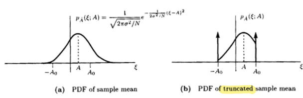
  • $\hat A=\bar x$ : MVUE, but can be outside of the range
  • $\check A=\begin{cases}-A_0,\;\bar x<-A_0\\\bar x,\;-A_0\leq\bar x\leq A_0\text{ : biased}\\A_0,\;\bar{x}>A_0\end{cases}$
    $p_A(\xi; A) = \Pr\{\bar{x} \leq -A_0\} \delta(\xi + A_0) \\+ p_A(\xi; A) [u(\xi + A_0) - u(\xi)] + \Pr\{\bar{x} \geq A_0\} \delta(\xi - A_0)$
    

---

• Mean squared error(MSE)
  $\text{mse}(\hat A)=\int^\infty_{-\infty}(\xi-A)^2 p_{\hat A}(\xi;A)d\xi\\[0.2cm] =\int^{-A_0}_{-\infty}(\xi-A)^2p_{\hat A}(\xi;A)d\xi+\int^{A_0}_{-A_0}(\xi-A)^2p_{\hat A}(\xi;A)d\xi+\int^\infty_{A_0}(\xi-A)^2p_{\hat A}(\xi;A)d\xi\\[0.2cm] >\int^{-A_0}_{-\infty}(-A_0-A)^2p_{\hat A}(\xi;A)d\xi+\int^{A_0}_{-A_0}(\xi-A)^2p_{\hat A}(\xi;A)d\xi+\int^\infty_{A_0}(A_0-A)^2p_{\hat A}(\xi;A)d\xi$
  • The truncated sample mean estimator $\check A$ is better than the sample mean estimator(MVUE) in terms of MSE
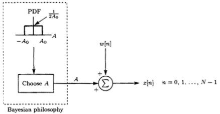
  • Using prior knowledge, $A$ is assumed to be a random variable, $A\sim U[-A_0,A_0]$
    → The problem is to estimate the value of $A$ or the realization of $A$
    

Bayesian MMSE Estimation

• Bayesian MSE(Bmse)
  $\text{Bmse}(\hat A)=E\left[(A-\hat A)^2\right],\text{ E w.r.t. the joint PDF }p(\text{x}, A)\\[0.2cm] =\int\int(A-\hat A)^2p(\text{x},A)d\text{x}dA=\int\left[\int(A-\hat A)^2p(A|\text{x})dA\right]p(\text{x})d\text{x}\\[0.2cm] \text{c.f., Classical MSE, mse}(\hat A)=\int(\hat A-A)^2p(\text{x};A)\text{x}$
• Bmse is minimized if $\int(A-\hat A)^2 p(A|\text{x})dA$ is minimized for each $\text{x}$
  $\frac{\partial}{\partial \hat A}\int(A-\hat A)^2 p(A|\text{x})dA=\int\frac{\partial}{\partial \hat A}(A-\hat A)^2 p(A|\text{x})dA\\[0.2cm] =\int-2(A-\hat A)p(A|\text{x})dA=-2\int Ap(A|\text{x})dA+2\hat A\int p(A|\text{x})dA=0\\[0.2cm] \int p(A|\text{x})dA = 1\\[0.2cm] \rightarrow \hat A=\int Ap(A|\text{x})dA=E(A|\text{x})\\[0.2cm] p(A|\text{x})=\frac{p(\text{x}|A)p(A)}{p(\text{x})}=\frac{p(\text{x}|A)p(A)}{\int p(\text{x}|A)p(A)dA}$
  

---

• Ex) DC Level in WGN
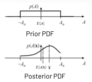
  $\prod^{N-1}_{n=0}p(x[n]|A)\\[0.2cm] p(\text{x}|A)=\frac{1}{(2\pi\sigma^2)^{N/2}}\exp\left[-\frac{1}{2\sigma^2}\sum^{N-1}_{n=0}(x[n]-A)^2\right],\;p(A)\sim U[-A_0,A_0]\\[0.3cm] \rightarrow p(A|\text{x})=\begin{cases} \frac{\frac{1}{2A_0(2\pi\sigma^2)^{N/2}}\exp\left[-\frac{1}{2\sigma^2}\sum^{N-1}_{n=0}(x[n]-A)^2\right]}{\int^{A_0}_{-A_0}\frac{1}{2A_0(2\pi\sigma^2)^{N/2}}\exp\left[-\frac{1}{2\sigma^2}\sum^{N-1}_{n=0}(x[n]-A)^2\right]dA},\;|A|\leq A_0\\ 0,\;|A|>A_0 \end{cases}\\[0.2cm] =\begin{cases} \frac{1}{c\sqrt{2\pi\sigma^2/N}}\exp\left[-\frac{1}{2\sigma^2/N}(A-\bar x)^2\right],\;|A|\leq A_0\\ 0,\;|A|> A_0 \end{cases}$

---

• $\hat A$ is a function of $\bar x$
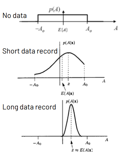
• MMSE estimator of $A$ before observing $\text{x}: \bar A =E(A)=0$
• The posterior mean lies between $0$ and $\bar x$
• As $N\rightarrow \infty,\;\bar A \rightarrow \bar x$
• In general, $\hat \theta= E(\theta|\text{x})=\int\theta p(\theta|\text{x})d\theta$
  

---

Choosing a Prior PDF

• Once a prior PDF has been chosen, the MMSE is
  $\hat \theta=E(\theta|\text{x})=\int\theta p(\theta|\text{x})d\theta,\;p(\theta|\text{x})=\frac{p(\text{x}|\theta)p(\theta)}{\int p(\text{x}|\theta)p(\theta)d\theta}$
  : usually difficult to obtain closed-form solution(numerical integration is needed
• Choice is crucial :
  • Must be able to justify it physically
  • Anything other than a Gaussian prior will likely result in no closed-form estimates
    (previous example showed a uniform prior led to a non-closed form,
    later exqmple shows a Gaussian prior gives a closed form)
  • There seems to be a trade-off between
    1. choosing the prior PDF as accurately as possible
    2. choosing the prior PDF to give computable closed form

---

Gaussian Prior PDF Example

• Ex) DC Level in WGN - Gaussian Prior PDF
  $p(A)=\frac{1}{\sqrt{2\pi\sigma_A^2}}\exp\left[-\frac{1}{2\sigma_A^2}(A-\mu_A)^2\right]\\[0.2cm] p(\text{x}|A)=\frac{1}{(2\pi\sigma^2)^{N/2}}\exp\left[-\frac{1}{2\sigma^2}\sum^{N-1}_{n=0}(x[n]-A)^2\right]\\[0.2cm] =\frac{1}{(2\pi\sigma^2)^{N/2}}\exp\left[-\frac{1}{2\sigma^2}\sum^{N-1}_{n=0}(x[n]-A)^2\right]\\[0.2cm] =\frac{1}{(2\pi\sigma^2)^{N/2}}\exp\left[-\frac{1}{2\sigma^2}\sum^{N-1}_{n=0}x^2[n]\right]\exp\left[-\frac{1}{2\sigma^2}(NA^2-2NA\bar x)\right]\\[0.3cm] p(A | \mathbf{x}) = \frac{p(\mathbf{x} | A)p(A)}{\int p(\mathbf{x} | A)p(A) \, dA} = \frac{\exp \left[ -\frac{1}{2} \left( \frac{1}{\sigma^2}(NA^2 - 2NA\bar{x}) + \frac{1}{\sigma_A^2}(A - \mu_A)^2 \right) \right]} {\int_{-\infty}^{\infty} \exp \left[ -\frac{1}{2} \left( \frac{1}{\sigma^2}(NA^2 - 2NA\bar{x}) + \frac{1}{\sigma_A^2}(A - \mu_A)^2 \right) \right] \, dA} \\[0.3cm]= \frac{\exp \left[ -\frac{1}{2} Q(A) \right]} {\int_{-\infty}^{\infty} \exp \left[ -\frac{1}{2} Q(A) \right] \, dA}\\[0.3cm] Q(A) = \frac{1}{\sigma^2} \left( N A^2 - 2 N A \bar{x} \right) + \frac{1}{\sigma_A^2} (A - \mu_A)^2\\[0.2cm] = \left( \frac{N}{\sigma^2} + \frac{1}{\sigma_A^2} \right) A^2- 2 \left( \frac{N}{\sigma^2} \bar{x} + \frac{\mu_A}{\sigma_A^2} \right) A+ \frac{\mu_A^2}{\sigma_A^2}\\[0.2cm] \rightarrow \begin{cases} \sigma_{A|\mathbf{x}}^2 = \frac{1}{\frac{N}{\sigma^2} + \frac{1}{\sigma_A^2}}\\ \mu_{A|\mathbf{x}} = \left( \frac{N}{\sigma^2} \bar{x} + \frac{\mu_A}{\sigma_A^2} \right) \sigma_{A|\mathbf{x}}^2 \end{cases}\\[0.2cm] p(A|\text{x})=\frac{1}{\sqrt{2\pi\sigma^2_{A|x}}}\exp\left[-\frac{1}{2\sigma^2_{A|x}}(A-\mu_{A|x})^2\right]$
  
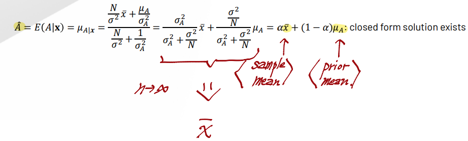
• As $N\rightarrow\infty,\;\alpha\rightarrow1,\;\hat A\rightarrow \bar x$
  $\text{var}(A|\text{x})=\sigma^2_{A|\text{x}}=\frac{1}{\frac{N}{\sigma^2}+\frac{1}{\sigma^2_A}}\\[0.2cm] \text{Bmse}(\hat A)=E\left[(A-\hat A)^2\right]=\int\int(A-\hat A)^2 p(\text{x};A)d\text{x}dA\\[0.2cm]=\int\left[\int(A-E(A|\text{x}))^2 p(A|\text{x})dA\right]p(\text{x})d\text{x}\\[0.2cm] =\int\text{var}(A|\text{x}) p(\text{x})d\text{x}=\frac{1}{\frac{N}{\sigma^2}+\frac{1}{\sigma^2_A}}=\frac{\sigma^2}{N}\left(\frac{\sigma^2_A}{\sigma^2_A+\frac{\sigma^2}{N}}\right)<\frac{\sigma^2}{N}$

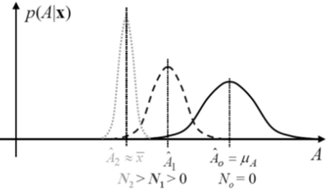
  improved performance with prior knowledge

• $p(\text{x}, A)$ Gaussian → $p(A),p(A|\text{x})$ Gaussian : reproducing property
  → Only mean and variance are recomputed

---

• Note
  • Closed-Form Solution for Estimate!
  • Estimate is weighted sum of prior mean & data mean
  • Weights balance between prior info quality and data quality
  • As $N$ increases...
    - Estimate $E(A|\text{x})$ moves $\mu_A\rightarrow \bar x$
    - Accuracy $\text{var}(A|\text{x})$ moves $\sigma^2_A\rightarrow\sigma^2/N$
    

    Gaussian Dat & Gaussian Prior gives Closed-Form MMSE Solution

---

Bivariate Gaussian PDF

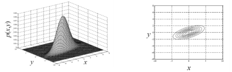
• If $x$ and $y$ are distributed according to a bivariate Gaussian PDF with
  mean vector $[E(x)\;E(y)]^T$, covariance matrix $\text{C}=\left[\begin{matrix}\text{var}(x) & \text{cov}(x,y)\\ \text{cov}(y,x)&\text{var}(y)\end{matrix}\right]$
  $\rightarrow p(x,y)=\frac{1}{2\pi\det^{\frac{1}{2}}(\text{C})}\exp\left[\begin{matrix} -\frac{1}{2} \left[\begin{matrix}x-E(x)\\y-E(y)\end{matrix}\right]^T&\text{C}^{-1}\left[\begin{matrix}x-E(x)\\y-E(y)\end{matrix}\right]\end{matrix}\right]$
  

---

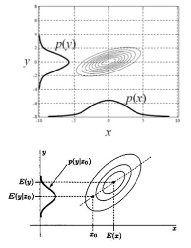
• The marginal (or individual) PDFs by integrating:
  $p(x)=\int^\infty_{-\infty}p(x,y)dy\\[0.2cm] p(y)=\int^\infty_{-\infty}p(x,y)dx$
• The conditional PDF $p(y|x)$ is also Gaussian and
  $E(y|x)=E(y)+\frac{\text{cov}(x,y)}{\text{var}(x)}(x-E(x))\\[0.2cm] \text{var}(y|x)=\text{var}(y)-\frac{\text{cov}^2(x,y)}{\text{var(x)}}$
  

---

• Prior PDF : $p(y)=N(E(y),\text{var}(y))$
  After observing $x$, the posterior PDF $p(y|x) =N(E(y|x), \text{var}(y|x))$
  $\text{var}(y|x)=\text{var}(y)\left[1-\frac{\text{cov}^2(x,y)}{\text{var}(x)\text{var}(y)}\right]=\text{var}(y)(1-\rho^2)$

  If $\rho$ is large then, variance reduction become larger

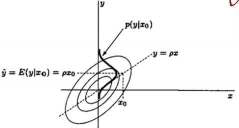
  $\rho=\frac{\text{cov}(x,y)}{\sqrt{\text{var}(x)\text{var}(y)}}:\text{correlation coefficient}\\[0.2cm] \hat y=E(y)+\frac{\text{cov}(x,y)}{\text{var}(x)}(x-E(x))\\[0.2cm] \rightarrow\hat y_n=\frac{\hat y-E(y)}{\sqrt {\text{var}(y)}}=\frac{\text{cov}(x,y)}{\sqrt{\text{var}(x)\text{var}(y)}}\frac{x-E(x)}{\sqrt{\text{var}(x)}}=\rho x_n$
  

---

Multivariate Gaussian PDF

• Let $\text{x}\;(k\times1)$ and $\text{y}\;(l\times1)$ are jointly Gaussian with $[E(\text{x})^T\;E(\text{y})^T]^T$ and
  $\text{C}=\left[\begin{matrix} C_{xx}&C_{xy}\\ C_{yx}&C_{yy}\end{matrix}\right]=\left[\begin{matrix} k\times k&k\times l\\ l\times k&l\times l\end{matrix}\right]$
  so that
  $p(\text{x},\text{y})=\frac{1}{(2\pi)^{\frac{k+l}{2}}\det^{\frac{1}{2}}(\text{C})}\exp \left[ - \frac{1}{2} \begin{pmatrix} \mathbf{x} - \mathbb{E}(\mathbf{x}) \\ \mathbf{y} - \mathbb{E}(\mathbf{y}) \end{pmatrix}^T \mathbf{C}^{-1} \begin{pmatrix} \mathbf{x} - \mathbb{E}(\mathbf{x}) \\ \mathbf{y} - \mathbb{E}(\mathbf{y}) \end{pmatrix} \right]$
  Then, $p(\text{y}|\text{x})$ is also Gaussian and,
  $E(\text{y}|\text{x})=E(\text{y})+C_{yx}C^{-1}_{xx}(\text{x}-E(\text{x}))\\ C_{y|x}=C_{yy}-C_{yx}C^{-1}_{xx}C_{xy}\\ E[\theta|x)=E[\theta]+C_{\theta x}C^{-1}_{xx}(x-E[x])$

All Content has been written based on lecture of Prof. eui-seok.Hwang in GIST(Detection and Estimation)