Overview
- Previously
- Introduced the idea of a
a priori information on θ→ use prior pdf: p(θ)
- Defined a new optimality criterion →
Bayesian MSE
- Showed the
Bmse is minimized by E(θ∣x), called mean of posterior pdf or conditional mean
- Now
- Define a more general optimality criterion
- leads to several different
Bayesian approaches
- includes
Bmse as special case
- Why?
- Provides flexibility in balancing: model, performance, and computations
Bayesian Risk Functions
- Previously, we used
Bmse as the Bayesian measure to minimizeBmse(θ^)=E[(θ−θ^)2]w.r.t.p(x,θ)→errorϵ=θ−θ^
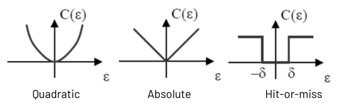
- In general, define a quadratic cost function, C(ϵ)=ϵ2=(θ−θ^)2
Bayes risk R : the average cost R=E[C(ϵ)]
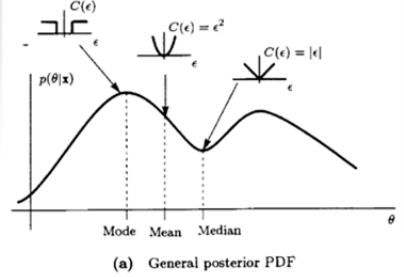
- Quadratic error : C(ϵ)=ϵ2
- Absolute error : C(ϵ)=∣ϵ∣
- Hit-ot-miss error : C(ϵ)={0,1,∣ϵ∣<δ∣ϵ∣>δ
R=E[C(ϵ)]=∫∫C(θ−θ^)p(x,θ)dxdθ=∫[∫C(θ−θ^)p(θ∣x)dθ]p(x)dx
minimize the inner integral
General Bayesian Estimators
- For a given desired cost function, find the form of the optimal estimator
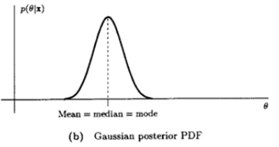
- Quadratic
R(θ^)=Bmse(θ^)=E[(θ−θ^)2]→θ^=E(θ∣x)=mean of p(θ∣x)
- Absolute
R(θ^)=E[∣θ−θ^∣]→θ^=median of p(θ∣x)
- Hit-or-Miss
θ^=mode of p(θ∣x)(max. a posterior, MAP)
Derivation for Absolute Cost Functiong(θ^)=∫∣θ−θ^∣p(θ∣x)dθ=∫−∞θ^(θ^−θ)p(θ∣x)dθ+∫θ^∞(θ^−θ)p(θ∣x)dθ - Set ∂θ^∂g(θ^)=0 and use Leibnitz's rule,
∂x∂(∫a(x)b(x)f(x,t)dt)=f(x,b(x))b′(x)−f(x,a(x))a′(x)+∫a(x)b(x)∂x∂f(x,t)dt
- 1st integral
f(θ^,θ)=(θ^−θ)p(θ∣x)→f(θ^,b(θ^))=0,a′(θ^)=0
- 2nd integral
f(θ^,θ)=(θ−θ^)p(θ∣x)→f(θ^,a(θ^))=0,b′(θ^)=0→∂θ^∂g(θ^)=∫−∞θ^p(θ∣x)dθ−∫θ^∞p(θ∣x)dθ=0→∫−∞θ^p(θ∣x)dθ=∫θ^∞p(θ∣x)dθ→θ^ is the median of the posterior PDF(Pr{θ≤θ^∣x}=21)
Derivation for Hit-or-Miss Cost Function
g(θ^)=∫−∞θ^−δ1⋅p(θ∣x)dθ+∫θ^+δ∞1⋅p(θ∣x)dθ=1−∫θ^−δθ^+δp(θ∣x)dθ
- Then Maximize
∫θ^−δθ^+δp(θ∣x)dθ
- For arbitrarily samll δ,θ^ corresponds to the location of
maximum or mode of the posterior PDF p(θ∣x)
maximum a posteriori (MAP) estimator
Minimum Mean Square Error Estimators
- For the scalar parameter case
θ^=E(θ∣x)=mean of p(θ∣x)
- Vector MMSE estimator
θ^=E(θ∣x) which minimizes the MSE
for each component of the unknown vector parameterE[(θi−θ^i)2]=∫(θi−θ^i)2p(θi∣x)dθiθ^i=∫∫θip(x,θ)dxdθ=E(θi∣x)θ^=[θ^1θ^2…θ^p]T=[E(θ1∣x)E(θ2∣x)…E(θp∣x)]T=E(θ∣x)
- Ex)
Bayesian Fourier analysis
- Signal model : x[n]=acos2πf0n+bsin2πf0n+w[n],n=0,1,⋯,N−1
where f0 is a multiple of 1/N except 0 or 21, w[n] is WGN with variance σ2θ=[ab]T with prior PDF θ∼N(0,σθ2I) common propagation model called Rayleigh Fadingx=Hθ+wH=⎣⎢⎢⎢⎢⎡1cos2πf0⋮cos[2πf0(N−1)]0sin2πf0⋮sin[2πf0(N−1)]⎦⎥⎥⎥⎥⎤
θ^=E(θ∣x)=σθ2HT(Hσθ2HT+σ2I)−1xCθ∣x=σθ2I−σθ2HT(Hσθ2HT+σ2I)−1Hσθ2
From μθ=0,Cθ=σθ2I,Cw=σ2I and multi-variate Gaussian results
E(y∣x)=E(y)+CyxCxx−1(x−E(x)),Cy∣x=Cyy−CyxCxx−1Cxy
Alternatively, using matrix inversion lemma,
θ^=E(θ∣x)=(σθ21I+HTσ21H)−1HTσ21xCθ∣x=(σθ21I+HTσ21H)−1
Since, HTH=2NI
θ^=(σθ21I+2σ2NI)−1HTσ21x=σθ21+2σ2Nσ21HTx⎩⎪⎪⎪⎨⎪⎪⎪⎧a^=1+σθ22σ2/N1[N2∑n=0N−1x[n]cos2πf0n]b^=1+σθ22σ2/N1[N2∑n=0N−1x[n]sin2πf0n],cθ∣x=σθ21+2σ2N1I→⎩⎪⎪⎨⎪⎪⎧Bmse(a^)=σθ21+2σ2N1Bmse(b^)=σθ21+2σ2N1
Properties of the MMSE Estimator
- Commutes over affine mappings(linearity):
α=Aθ+b→α^=E(α∣x)=E(Aθ+b∣x)=AE(θ∣x)+b=Aθ^+b
- Additive Property for independent data sets
θ^=E(θ∣x1,x2) θ,x1,x2 are jointly Gaussian and x1,x2 are independentLet x=[x1Tx2T]T from multi-variate Gaussian resultsθ^=E(θ∣x)=E(θ)+CθxCxx−1(x−E(x)),Cxx−1=[Cx1x1Cx2x1Cx1x2Cx2x2]−1=[Cx1x1−100Cx2x2−1]→θ^=E(θ)+[Cθx1Cθx2][Cx1x1−100Cx2x2−1][x1−E(x1)x2−E(x2)]=E(θ)+Cθx1Cx1x1−1(x1−E(x1))+Cθx2Cx2x2−1(x2−E(x2))
- Jointly Gaussian case leads to a linear estimator : θ^=Px+m
Maximum a Posteriori(MAP) Estimators
- Maximum a posteriori(MAP) estimators
θ^MAP=argθmaxp(θ∣x)→θ^MAP=argθmaxp(x∣θ)p(θ)→θ^MAP=argθmax[lnp(x∣θ)+lnp(θ)]
- Note : The "hit-or-miss" cost function gave the MAP estimator → it maximizes the posteriori PDF
- Given that the MMSE estimator is "the most natural" one, why the MAP estimator considered?
- If x and θ are not jointly Gaussian, the form for MMSE estimate requires integration to find the conditional mean. MAP avoids this computational problem (doesn't require this integration), trading "natural criterion(MMSE)" vs. "computational ease(MAP)"
- More flexibility to choose the prior PDF
- Ex) Exponential PDF
p(x[n]∣θ)={θexp(−θx[n]),0,x[n]>0x[n]<0,x[n]’s are conditional IIDp(x∣θ)=n=0∏N−1p(x[n]∣θ)The prior PDF, p(θ)={λexp(−λθ),0,θ>0θ<0 The MAP estimator is found by maximizingg(θ)=lnp(x∣θ)+lnp(θ)=Nlnθ−Nθxˉ+lnλ−λθ,θ>0dθdg(θ)=θN−Nxˉ−λ=0→θ^=xˉ+Nλ1As λ→0, the prior PDF becomes uniform. → Bayesian MLE.
Bayesian MLE
- As we keep getting good data, p(θ∣x) becomes more concentrated as a function of θ
But since:θ^MAP=argθmaxp(θ∣x)=argθmaxp(x∣θ)p(θ) p(x∣θ) should also become more concentrated as a function of θ
- Note that the prior PDF is nearly constant where p(x∣θ) is non-zero
- This becomes truer as N→∞ and p(x∣θ) gets more concentrated
→argθmaxp(θ∣x)≈argθmaxp(x∣θ)MAP≈Bayesian MLE 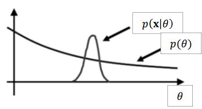
All Content has been written based on lecture of Prof. eui-seok.Hwang in GIST(Detection and Estimation)