Formal Description
Detection vs Estimation
Detection(Classification)
: Discrete set of hypotheses(right or wrong,
Classificationetc.)Estimation(Regression)
: Continuous set of hypotheses(almost always wrong -
minimize errorinstead)
Sort of Detection & Estimation
Classical: Fixed, non-random Hypotheses/parameters
Bayesian: Random, non-fixed Hypotheses/parametersBayesian problem assume priors or priori distributions
Mathematical Estimation Problem
Parameter estimation
-
From
discrete-timewaveform or data set, i.e.,N-point dataset depending onFixed(Deterministic)Classical Estimation
-
Mathematically model the data
probability density funcion(PDF)due to the randomness- :
;means it'sdeterministic
- :
-
Example assume that it's
Gaussian: denotes the mean, (N: Gaussian Normal Distribution) -
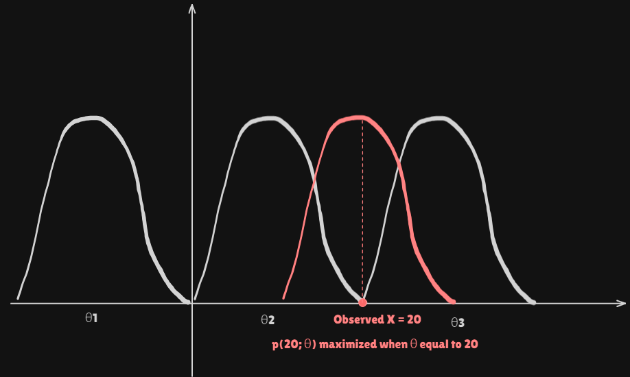
Infer the value of from the observed value of
- If
observed valueequal to20thanprobaility of observation20 maximized when is20.
- If
-
In actual problems,
PDF is not given but chosen- Consistent with constraints and prior knowledge
- Mathematically tractable
We don't know the actual distributionThe thing only we can do isGuess the distributionusing every background, knowledge etc.
-
Example : Dow-Jones industrial average
- :
White Guassian noise(WGN)White: i.i.dindependentandidentically distributed
- It can be just Product of marginal Probs because it'd White(iid)Why Gaussian?
Widely used and convience of calculation
CLT(Central Limit Theorem)
Add enough observations Follow
Gaussian Distribution
ForGuassianWhenWSS(Wide Sense Stationary)SSS(Stric Sence Stationary)
Types of estimation
Classical Estimation:Parametersof interest are assumed to beDeterministicBaysian Estimation:Parametersare assumed to beRandom Variablesto exploit any prior knowledge- Example : Average of Dow-Jones industrial average is in [2800, 3200]
background knowledge(prior)
- Example : Average of Dow-Jones industrial average is in [2800, 3200]
Estimator and Estimate
Estimator: Arule(Function)that assigns a value to for each realization ofFunction of Random Variable Random Variable
Function isEstimatorEstimate: The value of obtained for a given realization ofGetting value of into $ is
Estimation
Accessing Estimator Performance
Better Estimator? (Sample mean vs First sample value)
- Example of the DC level in noise
- : unknown DC level
target - : zero mean Gaussian process
- observations :
- Two candidate
estimators:Sample MeanvsFirst sample value
- Statiscal Analysis
MeanWe can switch and
Variance- What's better?
Sample meanis better estimator thanFirst valueEstimator Mean Variance Sample mean First value
Mathematical Detection Problem
Binary Hypothesis Test
Noise only hypothesisvs.signal present hypothesis(Deterministic signals)
- Example of the DC level in noise
: zero mean Gaussian process
- Which
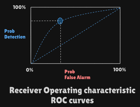
Detectoris better?
vs Receiver Operating Characteristic(ROC)curves- Probability of
false alarm(decide when istrue:Correct - Probability of
detection(decide when istrue:Wrong
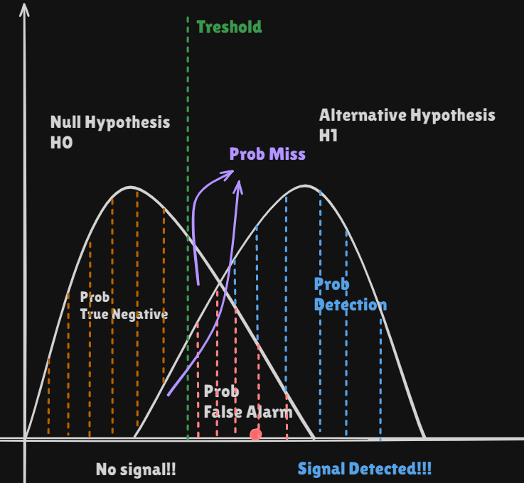
- Probability of
