Tabular task
This part of the blog covers how the tabular data can be handled for preprocessing, training and evaluation.
This work is most relavant to the example questions on AICE Associate course on the official website.
The work covers the line of example codes for solving the example questions and its variant according to my personal experience.
Setting up files as Dataframes
How to read json or csv files
import pandas as pd


DATA_PATH_json = './data/data.json'
DATA_PATH_csv = './data/data.csv'

df = pd.read_json("data.json")
df = pd.read_json(DATA_PATH_json)

# or

df = pd.read_csv("data.csv")
df = pd.read_json(DATA_PATH_csv)
Validating loaded files
How check or read nested json files
checking for nesting
import json

def is_nested(json_data):
    if isinstance(json_data, dict):
        for value in json_data.values():
            if isinstance(value, (dict, list)):
                return True
    return False

with open("data.json", "r") as file:
    data = json.load(file)

print(is_nested(data))


### How to observe the first few rows
print(df.head())
Dropping certain rows or columns
How to Drop Rows Where Address1 is '-'
df = df[df["Address1"] != "-"]

# or

df = df.drop(df[df["Address1"] == "-"].index)

# or

df = df.query("Address1 != '-'")
How to Drop Rows Where Address1 Contains Certain Values
df = df[~df["Address1"].isin(["-", "Unknown", "N/A"])]How to Drop Rows Based on a Condition in Multiple Columns
df = df[~((df["Address1"] == "-") & (df["City"] == "Seoul"))]How to use df.drop.na
# drop rows where...

# certain column
df = df.dropna(subset=["Column1"])

# certain multiple columns
df = df.dropna(subset=["Column1", "Column2"])

# any columns have null value
df = df.dropna()

# All columns of the rwo have null value
df = df.dropna(how="all")

# threshold% of columns have null values
threshold = 0.4  # 40% missing values
df = df[df["Column1"].isnull().mean() < threshold]
How to Drop Columns
# drop columns that all values are missing
df = df.dropna(axis=1, how="all")

# drop columns that have at least one missing value
df = df.dropna(axis=1)
How to Drop Rows Where Any Column Contains a Specific Value
df = df[~df.apply(lambda row: '-' in row.values, axis=1)]

# or

values_to_remove = ["-", "Unknown", "N/A"]

df = df[~df.apply(lambda row: any(val in row.values for val in values_to_remove), axis=1)]

 # or

# Drop Rows Where Any Column Contains Certain Values (Using isin())
values_to_remove = ["-", "Unknown", "N/A"]

df = df[~df.isin(values_to_remove).any(axis=1)]

 # or

# Drop Rows Where Specific Columns Contain Certain Values
columns_to_check = ["Column1", "Column2"]
values_to_remove = ["-", "Unknown", "N/A"]

df = df[~df[columns_to_check].isin(values_to_remove).any(axis=1)]

 # or

#  Drop Rows Where ALL Columns Contain Certain Values
values_to_remove = ["-", "Unknown", "N/A"]

df = df[~df.isin(values_to_remove).all(axis=1)]

 # or

# Drop Rows Where a Column Has More Than X% of Unwanted Values
threshold = 0.5  # 50% or more columns containing unwanted values
values_to_remove = ["-", "Unknown", "N/A"]

df = df[(df.isin(values_to_remove).sum(axis=1) / df.shape[1]) < threshold]
Counting the number of rows for cetain conditions
How to Count Rows Where Address1 is '-'
count = (df["Address1"] == "-").sum()
print("Number of rows with '-' as Address1:", count)
How to Count Rows Where Address1 is in a List of Values
count = df["Address1"].isin(["-", "Unknown", "N/A"]).sum()
print("Number of unwanted Address1 values:", count)
Merging dataframes into one with certain conditions
How to merge two/more dataframe using certain attribute
df_merged = pd.merge(df1, df2, on="RID", how="inner")df_merged = pd.merge(df1, df2, on="RID", how="inner")
df_merged = pd.merge(df_merged, df3, on="RID", how="inner")Dataframe shares same columns but have different rows (pd.concat axis=0)
df_merged = pd.concat([df1, df2, df3], axis=0, ignore_index=True)Dataframe shares same rows but have differenet colums (pd.concat axis=1)
They are merged according to the index
df_merged = pd.concat([df1, df2, df3], axis=1)Merging dataframe on mutliple keys
df_merged = pd.merge(df1, df2, on=["RID", "Date"], how="inner")Merging dataframe while the column names don't match
df_merged = pd.merge(df1, df2, left_on="ID", right_on="RID", how="inner")Preserving all data from both DataFrames (keeps all records even if some RID values are missing in either DataFrames)
df_merged = pd.merge(df1, df2, on="RID", how="outer")One-Hot encoding or Categorical Labeling
One-Hot encoding
What is One-Hot encoding?
One-Hot encoding involves converting categorical variable(columns in a dataframe) into numerical representations of 0 or 1
One-Hot encoding using Pandas
Basic one-hot encoding
In Pandas, the object datatype is a flexible type that typically stores strings, but it can also hold mixed types (numbers, lists, or even dictionaries).
import pandas as pd

df = pd.DataFrame({
    "A": ["apple", "banana", "cherry"],  # Strings
    "B": [1, 2, 3],  # Integers
    "C": [3.14, 2.71, 1.61],  # Floats
    "D": ["1", "2", "3"]  # Numbers stored as strings
})
object_columns = df.select_dtypes(include=["object"]).columns
print("Object columns:", object_columns)

# Object columns: Index(['A', 'D'], dtype='object')


#####################################################################
df_encoded = pd.get_dummies(df, columns=df.select_dtypes(include=["object"]).columns)
#####################################################################
Instructions for changing data type in pandas
Even though Pandas stores text data as object, you can explicitly convert it to str:
df["A"] = df["A"].astype(str)Sometimes, object columns contain numeric values as strings:
df["D"] = df["D"].astype(int) # Converts "1", "2", "3" to integersOne-Hot Encoding for Specific Columns
df_encoded = pd.get_dummies(df, columns=["Column1", "Column2"])
# Encodes only Column1 and Column2, leaving other columns unchanged.
One-Hot Encoding While Keeping the Original Columns
df_encoded = df.copy()
df_encoded = pd.get_dummies(df_encoded, columns=["Category"], prefix="Category", drop_first=False)
# Keeps the original categorical column and adds one-hot-encoded features.
One-Hot Encoding with drop_first=True (Avoid Dummy Variable Trap)
df_encoded = pd.get_dummies(df, columns=["Category"], drop_first=True)
# Drops the first category in each one-hot encoding. Useful for regression models to prevent multicollinearity (dummy variable trap).
One-Hot Encoding with custom prefix
df_encoded = pd.get_dummies(df, columns=["Category"], prefix="Cat")
# Encodes Category but uses "Cat_" as a prefix for the new columns.
   Cat_A  Cat_B  Cat_C
0      1      0      0
1      0      1      0
2      0      0      1
🔹 What is the Dummy Variable Trap?
The Dummy Variable Trap is a problem that occurs when using one-hot encoding (pd.get_dummies(), OneHotEncoder()) where one categorical variable is perfectly predicted by the others, causing multicollinearity in regression models.
import pandas as pd

df = pd.DataFrame({"Color": ["Red", "Green", "Blue", "Red", "Blue"]})
df_encoded = pd.get_dummies(df, columns=["Color"])
print(df_encoded)

   Color_Blue  Color_Green  Color_Red
0          0            0         1
1          0            1         0
2          1            0         0
3          0            0         1
4          1            0         0
🔹 Why is This a Problem?
The Color_Red column is redundant because if Color_Blue = 0 and Color_Green = 0, then Color_Red must be 1.
This creates perfect multicollinearity, meaning one feature can be predicted from the others, leading to unstable regression models.
✅ 2. How to Avoid the Dummy Variable Trap
df_encoded = pd.get_dummies(df, columns=["Color"], drop_first=True)
print(df_encoded)

# or

from sklearn.preprocessing import OneHotEncoder

encoder = OneHotEncoder(drop="first", sparse_output=False)
df_encoded = encoder.fit_transform(df)

   Color_Blue  Color_Green
0          0            0
1          0            1
2          1            0
3          0            0
4          1            0
🔹 Now, "Color_Red" is removed, preventing redundancy and multicollinearity.
✅ 3. When is the Dummy Variable Trap a Problem?
Linear Models (Linear Regression, Logistic Regression, SVM, etc.)
🚨 Yes, it affects them.
Tree-Based Models (Decision Trees, Random Forests, XGBoost, etc.)
✅ No, they don't suffer from multicollinearity.
One-Hot encoding using sklearn OneHotEncoder()
✅ 1. Basic One-Hot Encoding
Encodes categorical variables into binary columns.
from sklearn.preprocessing import OneHotEncoder
import pandas as pd

df = pd.DataFrame({"Color": ["Red", "Green", "Blue", "Red", "Blue"]})

encoder = OneHotEncoder(sparse_output=False)
encoded = encoder.fit_transform(df)

df_encoded = pd.DataFrame(encoded, columns=encoder.get_feature_names_out(["Color"]))
print(df_encoded)

   Color_Blue  Color_Green  Color_Red
0        0.0         0.0       1.0
1        0.0         1.0       0.0
2        1.0         0.0       0.0
3        0.0         0.0       1.0
4        1.0         0.0       0.0
✅ 2. Avoiding the Dummy Variable Trap (drop="first")
Drops the first category to prevent multicollinearity in regression models.
from sklearn.preprocessing import OneHotEncoder
import pandas as pd

encoder = OneHotEncoder(drop="first", sparse_output=False)
encoded = encoder.fit_transform(df)

df_encoded = pd.DataFrame(encoded, columns=encoder.get_feature_names_out(["Color"]))
print(df_encoded)

   Color_Blue  Color_Green
0        0.0         0.0
1        0.0         1.0
2        1.0         0.0
3        0.0         0.0
4        1.0         0.0
🔹 Removes Color_Red, preventing the Dummy Variable Trap.
✅ 3. Handling Unknown Categories (handle_unknown="ignore")
When new categories appear in test data, the model won’t break.
from sklearn.preprocessing import OneHotEncoder
import pandas as pd

encoder = OneHotEncoder(handle_unknown="ignore", sparse_output=False)
encoded = encoder.fit_transform(df)

# Simulate new test data
df_test = pd.DataFrame({"Color": ["Red", "Purple"]})
encoded_test = encoder.transform(df_test)

df_test_encoded = pd.DataFrame(encoded_test, columns=encoder.get_feature_names_out(["Color"]))
print(df_test_encoded)

   Color_Blue  Color_Green  Color_Red
0        0.0         0.0       1.0
1        0.0         0.0       0.0
🔹 handle_unknown="ignore" ensures "Purple" doesn't break the model—it gets all zeros.
✅ 4. Encoding Multiple Columns
Encodes multiple categorical columns.
from sklearn.preprocessing import OneHotEncoder
import pandas as pd

df = pd.DataFrame({
    "Color": ["Red", "Green", "Blue", "Red"],
    "Size": ["Small", "Medium", "Large", "Small"]
})

encoder = OneHotEncoder(sparse_output=False)
encoded = encoder.fit_transform(df)

df_encoded = pd.DataFrame(encoded, columns=encoder.get_feature_names_out(df.columns))
print(df_encoded)

   Color_Blue  Color_Green  Color_Red  Size_Large  Size_Medium  Size_Small
0        0.0         0.0       1.0        0.0        0.0        1.0
1        0.0         1.0       0.0        0.0        1.0        0.0
2        1.0         0.0       0.0        1.0        0.0        0.0
3        0.0         0.0       1.0        0.0        0.0        1.0
LabelEncoder() converts categorical values into integers that ML modles understand
✅ 1. Basic Usage of LabelEncoder()
Converts categorical values into unique integer labels.
from sklearn.preprocessing import LabelEncoder
import pandas as pd

df = pd.DataFrame({"Color": ["Red", "Green", "Blue", "Red", "Blue"]})

encoder = LabelEncoder()  # Initialize encoder
df["Color_encoded"] = encoder.fit_transform(df["Color"])  # Fit and transform

print(df)

   Color  Color_encoded
0    Red              2
1  Green              1
2   Blue              0
3    Red              2
4   Blue              0
✅ 2. Encoding Multiple Columns with apply()
Instead of encoding a single column, encode multiple categorical columns.
df = pd.DataFrame({
    "Color": ["Red", "Green", "Blue", "Red"],
    "Size": ["Small", "Medium", "Large", "Small"]
})

encoder = LabelEncoder()

for col in ["Color", "Size"]:
    df[col + "_encoded"] = encoder.fit_transform(df[col])

print(df)

   Color    Size  Color_encoded  Size_encoded
0    Red   Small              2             2
1  Green  Medium              1             1
2   Blue   Large              0             0
3    Red   Small              2             2
🔹 Applies LabelEncoder() to multiple columns using a loop.
✅ 3. Converting Encoded Values Back to Original Labels
Instead of encoding a single column, encode multiple categorical columns.
df["Color_original"] = encoder.inverse_transform(df["Color_encoded"])
print(df)

   Color  Color_encoded Color_original
0    Red              2            Red
1  Green              1          Green
2   Blue              0           Blue
3    Red              2            Red
🔹 Recovers the original labels from their encoded values.
(번외) Try multi-class classification task with randomforest using LabelEncoder
✅ Step 1: Prepare Multi-Class Data
import pandas as pd
from sklearn.preprocessing import LabelEncoder
from sklearn.model_selection import train_test_split
from sklearn.ensemble import RandomForestClassifier
from sklearn.metrics import accuracy_score

# Sample dataset: Fruit classification (multi-class problem)
df = pd.DataFrame({
    "Weight": [150, 120, 130, 180, 160, 140, 170, 200],
    "Size": [7, 6, 6, 8, 7, 6, 7, 9],
    "Fruit": ["Apple", "Banana", "Apple", "Cherry", "Banana", "Apple", "Cherry", "Cherry"]
})

print(df)

   Weight  Size   Fruit
0     150     7  Apple
1     120     6  Banana
2     130     6  Apple
3     180     8  Cherry
4     160     7  Banana
5     140     6  Apple
6     170     7  Cherry
7     200     9  Cherry
✅ Step 2: Encode the Target Variable (Fruit) Using LabelEncoder
encoder = LabelEncoder()

# Transform categorical target labels into numerical labels
df["Fruit_encoded"] = encoder.fit_transform(df["Fruit"])

print(df)
   Weight  Size   Fruit  Fruit_encoded
0     150     7  Apple              0
1     120     6  Banana             1
2     130     6  Apple              0
3     180     8  Cherry             2
4     160     7  Banana             1
5     140     6  Apple              0
6     170     7  Cherry             2
7     200     9  Cherry             2

"Apple"  → 0
"Banana" → 1
"Cherry" → 2
✅ Step 3: Train a Multi-Class Classifier
Now, we use Fruit_encoded as the target variable (y) in classification.
# Define features (X) and target (y)
X = df[["Weight", "Size"]]
y = df["Fruit_encoded"]

# Split dataset into training and testing sets (80-20 split)
X_train, X_test, y_train, y_test = train_test_split(X, y, test_size=0.2, random_state=42)

# Train a Random Forest Classifier
clf = RandomForestClassifier(n_estimators=100, random_state=42)
clf.fit(X_train, y_train)

# Predict on test data
y_pred = clf.predict(X_test)

# Evaluate the model
accuracy = accuracy_score(y_test, y_pred)
print(f"Accuracy: {accuracy:.2f}")

Accuracy: 1.00
✅ Step 4: Decode Predictions Back to Original Labels
Once the model makes predictions (y_pred), we can convert the numerical labels back to categorical names.
y_pred_labels = encoder.inverse_transform(y_pred)
print(y_pred_labels)

['Cherry' 'Apple']
Let's get back on track!
How to Split Data Into Train and Validation Sets (train_test_split)
✅ 1. Basic Usage of train_test_split
from sklearn.model_selection import train_test_split

X = df.drop(columns=["Time_Driving"])  # Features
y = df["Time_Driving"]  # Target

X_train, X_test, y_train, y_test = train_test_split(X, y, test_size=0.2, random_state=42)
✅ This method prevents overfitting by ensuring that the model is tested on unseen data.
✅ 2. Splitting Data Into Train, Validation, and Test Sets
Instead of just train-test split, it's common to have a validation set for model tuning.
# First, split into Train (80%) and Test (20%)
X_train, X_test, y_train, y_test = train_test_split(X, y, test_size=0.2, random_state=42)

# Further split Train into Train (80%) and Validation (20%)
X_train, X_val, y_train, y_val = train_test_split(X_train, y_train, test_size=0.2, random_state=42)
- Train: 64%
- Validation: 16%
- Test: 20%
🔹 Explanation
Step 1: Split X and y into X_train (80%) and X_test (20%).
Step 2: Further split X_train into X_train (64%) and X_val (16%) for validation.
🔹 Why use a validation set?
Helps tune hyperparameters before testing on unseen data.
Prevents overfitting to the test set.
Used for early stopping in deep learning models.
✅ 3. Using Stratified Splitting for Imbalanced Datasets
For classification tasks with imbalanced classes, ensure that both training and test sets maintain class proportions.
X_train, X_test, y_train, y_test = train_test_split(
    X, y, test_size=0.2, random_state=42, stratify=y
)
🔹 Explanation
stratify=y ensures that the class distribution is preserved in both sets.
Useful when dealing with imbalanced data (e.g., fraud detection, medical diagnosis).
✅ Example Use Case: If y contains 90% class A and 10% class B, stratify=y ensures that the split retains this ratio.
✅ 4. Using K-Fold Cross-Validation Instead of a Fixed Train-Test Split
Instead of splitting once, cross-validation repeatedly trains on different splits of data.
from sklearn.model_selection import KFold

kf = KFold(n_splits=5, shuffle=True, random_state=42)

for train_index, test_index in kf.split(X):
    X_train, X_test = X.iloc[train_index], X.iloc[test_index]
    y_train, y_test = y.iloc[train_index], y.iloc[test_index]
🔹 Explanation
n_splits=5: Splits the data into 5 different train-test sets.
shuffle=True: Ensures randomization of data.
The model trains and tests on different subsets, improving generalization.
✅ Best for: Small datasets where a single train-test split may not be representative.
Full code example for K-fold cross validation using randomforest
import numpy as np
import pandas as pd
from sklearn.model_selection import KFold
from sklearn.ensemble import RandomForestClassifier
from sklearn.metrics import accuracy_score

# 🔹 Step 1: Create a Sample Dataset
df = pd.DataFrame({
    "Feature1": [2, 3, 5, 7, 9, 10, 11, 13, 15, 18],
    "Feature2": [1, 4, 6, 8, 10, 12, 14, 16, 17, 20],
    "Target":    [0, 1, 0, 1, 0, 1, 0, 1, 0, 1]  # Binary classification
})

X = df.drop(columns=["Target"])  # Features
y = df["Target"]  # Target variable

# 🔹 Step 2: Initialize K-Fold Cross-Validation
kf = KFold(n_splits=5, shuffle=True, random_state=42)

# Store results
accuracies = []

# 🔹 Step 3: Perform K-Fold Cross-Validation
for train_index, test_index in kf.split(X):
    # Split into training and testing sets
    X_train, X_test = X.iloc[train_index], X.iloc[test_index]
    y_train, y_test = y.iloc[train_index], y.iloc[test_index]

    # Initialize the RandomForestClassifier
    model = RandomForestClassifier(n_estimators=100, random_state=42)

    # Train the model
    model.fit(X_train, y_train)

    # Make predictions
    y_pred = model.predict(X_test)

    # Evaluate accuracy
    accuracy = accuracy_score(y_test, y_pred)
    accuracies.append(accuracy)

    print(f"Fold Accuracy: {accuracy:.4f}")

# 🔹 Step 4: Compute Average Accuracy Across Folds
average_accuracy = np.mean(accuracies)
print(f"\nAverage K-Fold Accuracy: {average_accuracy:.4f}")

Fold Accuracy: 1.0000
Fold Accuracy: 1.0000
Fold Accuracy: 0.5000
Fold Accuracy: 1.0000
Fold Accuracy: 1.0000

Average K-Fold Accuracy: 0.9000
🔹 Explanation
Create Dataset (df) → Includes 2 features and binary target (0 or 1).
Split Data (KFold(n_splits=5)) → Divides the dataset into 5 folds.
Train Model (RandomForestClassifier()) → Trains a new Random Forest model in each fold.
Evaluate Accuracy (accuracy_score()) → Measures model performance in each fold.
Compute Average Accuracy → Gets the overall model performance.
🚀 Use K-Fold CV to ensure your model generalizes well across different subsets of data!
Would you like a Stratified K-Fold example for imbalanced datasets? 🎯
Let's get back on track!
How to scale feature so it is suitable for training
First, verify what scaler functions is suitable!
The best scaler depends on the dataset:
If data is normally distributed → Use StandardScaler.
If data has many outliers → Use RobustScaler.
If data needs to be bounded (0-1) → Use MinMaxScaler.
✅ Step 1: Create a Sample DataFrame
import numpy as np
import pandas as pd

# Sample dataset with outliers
data = {
    "Feature1": [10, 200, 30, 400, 50, 600, 20, 700, 40, 1000],  # Outliers present
    "Feature2": [5, 500, 15, 700, 25, 800, 35, 900, 45, 1000],   # Outliers present
}

df = pd.DataFrame(data)

# Display original statistics
print("Before Scaling:\n", df.describe())
✅ Why include describe()?
Shows mean, standard deviation, min, max, and quartiles.
Helps identify outliers that may influence scaling.
✅ Step 2: Apply Different Scalers
from sklearn.preprocessing import StandardScaler, MinMaxScaler, RobustScaler

# Initialize scalers
scalers = {
    "StandardScaler": StandardScaler(),
    "MinMaxScaler": MinMaxScaler(),
    "RobustScaler": RobustScaler()
}

# Apply each scaler and store results
scaled_dfs = {}

for scaler_name, scaler in scalers.items():
    scaled_dfs[scaler_name] = pd.DataFrame(scaler.fit_transform(df), columns=df.columns)
    print(f"\nAfter {scaler_name}:\n", scaled_dfs[scaler_name].describe())
✅ How this helps?
Compare min, max, and quartiles to see how scaling affects values.
Check if outliers still dominate (e.g., StandardScaler is affected by extreme values).
✅ RobustScaler() - Scaling Train and Test Separately
To prevent data leakage, fit RobustScaler only on the training data and apply it to the test data.
from sklearn.model_selection import train_test_split

# Split data
X_train, X_test = train_test_split(df, test_size=0.2, random_state=42)

# Fit only on training data
scaler = RobustScaler()
X_train_scaled = scaler.fit_transform(X_train)

# Apply the same scaler to test data
X_test_scaled = scaler.transform(X_test)
✅ Why?
If you fit the scaler on the full dataset, it may leak information from the test set.
Always fit on X_train and transform both X_train & X_test.
✅ StandardScaler (Mean & Std)
✅ Good for normally distributed data, but sensitive to outliers.
from sklearn.preprocessing import StandardScaler

scaler = StandardScaler()
df_scaled = scaler.fit_transform(df)
✅ MinMaxScaler (Min-Max Scaling)
✅ Scales data between 0 and 1 but is affected by outliers.
from sklearn.preprocessing import MinMaxScaler

scaler = MinMaxScaler()
df_scaled = scaler.fit_transform(df)
✅ MaxAbsScaler (Absolute Maximum Scaling)
✅ Best for sparse data where values are positive and large.
from sklearn.preprocessing import MaxAbsScaler

scaler = MaxAbsScaler()
df_scaled = scaler.fit_transform(df)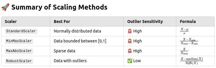
Back on Track!
Logistic Regression (로지스틱 회귀, 분류)
LogisticRegression
Logistic Regression을 사용하기 위해서는 로드하는 과정이 필요하다.
C: 규제 강도
max_iter: 반복 횟수
# import
from sklearn.linear_model import LogisticRegression

# 모델 생성
lg = LogisticRegression(C=1.0, max_iter=1000)

# 모델 학습
lg.fit(X_train, y_train)

# 모델 평가
lg.score(X_test, y_test)
Decision Tree (의사결정 나무, 분류/회귀)
DecisionTreeClassifier / DecisionTreeRegressor
Decision Tree를 사용하기 위해서는 로드하는 과정이 필요하다.
max_depth: 트리 깊이
random_state: 랜덤 시드
# import
from sklearn.tree import DecisionTreeClassifier # 분류
from sklearn.tree import DecisionTreeRegressor # 회귀

# 모델 생성
dt = DecisionTreeClassifier(max_depth=5, random_state=2023)

# 모델 학습
dt.fit(X_train, y_train)

# 모델 평가
dt.score(X_test, y_test)
Random Forest (랜덤 포레스트, 분류/회귀)
RandomForestClassifier / RandomForestRegressor
Random Forest를 사용하기 위해서는 로드하는 과정이 필요하다.
n_estimators: 사용하는 트리 개수
random_state: 랜덤 시드
# import
from sklearn.ensemble import RandomForestClassifier # 분류
from sklearn.ensemble import RandomForestRegressor # 회귀

# 모델 생성
rf = RandomForestClassifier(n_estimators=100, random_state=2023)

# 모델 학습
rf.fit(X_train, y_train)

# 모델 평가
rf.score(X_test, y_test)
XGBoost (분류/회귀)
XGBClassifier / XGBRegressor
XGBoost를 사용하기 위해서는 설치 및 로드하는 과정이 필요하다.
n_estimators: 사용하는 트리 개수
# install
!pip install xgboost

# import
from xgboost import XGBClassifier # 분류
from xgboost import XGBRegressor # 회귀

# 모델 생성
xgb = XGBClassifier(n_estimators=100)

# 모델 학습
xgb.fit(X_train, y_train)

# 모델 평가
xgb.score(X_test, y_test)
Light GBM (분류/회귀)
LGBMClassifier / LGBMRegressor
Light GBM을 사용하기 위해서는 설치 및 로드하는 과정이 필요하다.
n_estimators: 사용하는 트리 개수
# install
!pip install lightgbm

# import
from lightgbm import LGBMClassifier # 분류
from lightgbm import LGBMegressor # 회귀

# 모델 생성
lgbm = LGBMClassifier(n_estimators=100)

# 모델 학습
lgbm.fit(X_train, y_train)

# 모델 평가
lgbm.score(X_test, y_test)
Model prediction
predict()
# 모델 예측
model.predict(X_test)
Model Validation
regression model: MSE, RMSE, MAE, ...
classfication model: Accuracy, Precision, Recall, F1 Score, ...
# import
from sklearn.metrics import * # 모든 함수 로드

# 분류 모델 평가 지표
from sklearn.metrics import accuracy_score 		# 정확도
from sklearn.metrics import precision_score 	# 정밀도
from sklearn.metrics import recall_score 		# 재현율
from sklearn.metrics import f1_score 			# f1 score
from sklearn.metrics import confusion_matrix 	# 혼동행렬
from sklearn.metrics import accuracy_score 		# 모든 지표 한번에

# 회귀 모델 평가 지표
from sklearn.metrics import r2_score			# R2 결정계수
from sklearn.metrics import mean_squared_error	# MSE
from sklearn.metrics import mean_absolute_error	# MAE


# Example usage for classification
accuracy = accuracy_score(y_test, y_pred)
precision = precision_score(y_test, y_pred, average='macro')  # Use 'macro' for multi-class
recall = recall_score(y_test, y_pred, average='macro')
f1 = f1_score(y_test, y_pred, average='macro')
cf_matrix = confusion_matrix(y_test, y_pred)

# Print results
print(f"Accuracy: {accuracy:.4f}")
print(f"Precision: {precision:.4f}")
print(f"Recall: {recall:.4f}")
print(f"F1 Score: {f1:.4f}")
print(f"Confusion Matrix:\n{cf_matrix}")
✅ Explanation:
average='macro' → Used for multi-class classification.
confusion_matrix() → Returns a matrix of actual vs. predicted values.
🔹 Confusion Matrix Visualization (Heatmap)
import seaborn as sns
import matplotlib.pyplot as plt

sns.heatmap(cf_matrix, annot=True, fmt='d', cmap='Blues')  # Visualize confusion matrix
plt.xlabel("Predicted Label")
plt.ylabel("True Label")
plt.title("Confusion Matrix")
plt.show()
✅ Why?
Helps identify misclassified examples in classification tasks.
🔹 Regression Metrics (for y_test and y_pred)
from sklearn.metrics import r2_score, mean_squared_error, mean_absolute_error

# Example usage for regression
r2 = r2_score(y_test, y_pred)
mse = mean_squared_error(y_test, y_pred)
mae = mean_absolute_error(y_test, y_pred)

# Print results
print(f"R² Score: {r2:.4f}")
print(f"Mean Squared Error (MSE): {mse:.4f}")
print(f"Mean Absolute Error (MAE): {mae:.4f}")
✅ Explanation:
r2_score() → Measures how well the model explains variance in data.
mean_squared_error() → Penalizes large errors (better for big errors).
mean_absolute_error() → Measures absolute error size (better for interpretation).
In the end this is an example code
How to Train a Decision Tree & Random Forest
from sklearn.tree import DecisionTreeRegressor
from sklearn.ensemble import RandomForestRegressor

dt = DecisionTreeRegressor(max_depth=5, min_samples_split=3, random_state=120)
dt.fit(X_train, y_train)

rf = RandomForestRegressor(max_depth=5, min_samples_split=3, random_state=120, n_estimators=100)
rf.fit(X_train, y_train)
How to Compute Mean Absolute Error (MAE)
from sklearn.metrics import mean_absolute_error

y_pred_dt = dt.predict(X_test)
y_pred_rf = rf.predict(X_test)

mae_dt = mean_absolute_error(y_test, y_pred_dt)
mae_rf = mean_absolute_error(y_test, y_pred_rf)

print("Decision Tree MAE:", mae_dt)
print("Random Forest MAE:", mae_rf)
Now! finally Nerual Network for Tabular Task
For Binary Classification
How to Train a Neural Network with PyTorch
import torch
import torch.nn as nn
import torch.optim as optim
from torch.utils.data import DataLoader, TensorDataset

# Convert Data to Tensors
X_train_tensor = torch.tensor(X_train, dtype=torch.float32)
y_train_tensor = torch.tensor(y_train.values, dtype=torch.float32).view(-1, 1)  # Ensure float for BCEWithLogitsLoss
X_valid_tensor = torch.tensor(X_test, dtype=torch.float32)
y_valid_tensor = torch.tensor(y_test.values, dtype=torch.float32).view(-1, 1)

# Create DataLoaders
train_dataset = TensorDataset(X_train_tensor, y_train_tensor)
valid_dataset = TensorDataset(X_valid_tensor, y_valid_tensor)

train_loader = DataLoader(train_dataset, batch_size=16, shuffle=True)
valid_loader = DataLoader(valid_dataset, batch_size=16, shuffle=False)

# Define Binary Classification Neural Network
class BinaryClassifier(nn.Module):
    def __init__(self, input_size):
        super(BinaryClassifier, self).__init__()
        self.model = nn.Sequential(
            nn.Linear(input_size, 64),
            nn.ReLU(),
            nn.Linear(64, 32),
            nn.ReLU(),
            nn.Dropout(0.2),
            nn.Linear(32, 1),  # Single output neuron for binary classification
            nn.Sigmoid()  # Sigmoid activation to output probabilities (0 to 1)
        )

    def forward(self, x):
        return self.model(x)

# Initialize Model, Loss Function, and Optimizer
input_size = X_train.shape[1]
model = BinaryClassifier(input_size)

criterion = nn.BCELoss()  # Binary Cross-Entropy Loss
optimizer = optim.Adam(model.parameters(), lr=0.001)

# Training Loop
epochs = 30
history = {"train_loss": [], "valid_loss": []}

device = torch.device("cuda" if torch.cuda.is_available() else "cpu")
model.to(device)

for epoch in range(epochs):
    model.train()
    train_loss = 0

    for X_batch, y_batch in train_loader:
        X_batch, y_batch = X_batch.to(device), y_batch.to(device)
        y_pred = model(X_batch)
        loss = criterion(y_pred, y_batch)

        optimizer.zero_grad()
        loss.backward()
        optimizer.step()

        train_loss += loss.item()

    train_loss /= len(train_loader)
    history["train_loss"].append(train_loss)

    model.eval()
    valid_loss = 0

    with torch.no_grad():
        for X_batch, y_batch in valid_loader:
            X_batch, y_batch = X_batch.to(device), y_batch.to(device)
            y_pred = model(X_batch)
            loss = criterion(y_pred, y_batch)
            valid_loss += loss.item()

    valid_loss /= len(valid_loader)
    history["valid_loss"].append(valid_loss)

    print(f"Epoch {epoch+1}/{epochs} - Train Loss: {train_loss:.4f}, Validation Loss: {valid_loss:.4f}")

print("Training Complete!")


# how to used the model for evaluation

model.eval()
with torch.no_grad():
    y_pred = model(X_valid_tensor.to(device))

# Convert probabilities to binary labels (0 or 1)
y_pred_binary = (y_pred.cpu().numpy() > 0.5).astype(int)
print(y_pred_binary)
🔹 How to Train a Neural Network with TensorFlow (Equivalent to PyTorch Code)
import tensorflow as tf
from tensorflow import keras
from tensorflow.keras import layers
from sklearn.model_selection import train_test_split
import numpy as np

# Split Data (Make sure y contains binary labels: 0 or 1)
X_train_np, X_valid_np, y_train_np, y_valid_np = train_test_split(X, y, test_size=0.2, random_state=42)

# Convert Data to TensorFlow Tensors
X_train_tf = tf.convert_to_tensor(X_train_np, dtype=tf.float32)
y_train_tf = tf.convert_to_tensor(y_train_np.values.reshape(-1, 1), dtype=tf.float32)
X_valid_tf = tf.convert_to_tensor(X_valid_np, dtype=tf.float32)
y_valid_tf = tf.convert_to_tensor(y_valid_np.values.reshape(-1, 1), dtype=tf.float32)

# Create TensorFlow Dataset for Batching
batch_size = 16
train_dataset = tf.data.Dataset.from_tensor_slices((X_train_tf, y_train_tf)).shuffle(1024).batch(batch_size)
valid_dataset = tf.data.Dataset.from_tensor_slices((X_valid_tf, y_valid_tf)).batch(batch_size)

# Define Binary Classification Neural Network
model = keras.Sequential([
    layers.Dense(64, activation="relu", input_shape=(X_train.shape[1],)),
    layers.Dense(32, activation="relu"),
    layers.Dropout(0.2),
    layers.Dense(1, activation="sigmoid")  # Sigmoid activation for binary classification
])

# Compile Model with Binary Cross-Entropy Loss
model.compile(
    optimizer=keras.optimizers.Adam(learning_rate=0.001),
    loss="binary_crossentropy",  # Correct loss function for binary classification
    metrics=["accuracy"]  # Track accuracy during training
)

# Train the Model
epochs = 30
history = model.fit(
    train_dataset,
    validation_data=valid_dataset,
    epochs=epochs,
    verbose=1
)

print("Training Complete!")


#✅ Making Predictions and Converting to Binary Labels
# Predict on validation set
y_pred_probs = model.predict(X_valid_tf)

# Convert probabilities to binary labels (0 or 1)
y_pred_binary = (y_pred_probs > 0.5).astype(int)

print(y_pred_binary[:10])  # Show first 10 prediction
How to Plot Training and Validation Loss
import matplotlib.pyplot as plt

epochs = range(1, len(history["train_loss"]) + 1)

plt.plot(epochs, history["train_loss"], label="Train Loss", marker="o")
plt.plot(epochs, history["valid_loss"], label="Validation Loss", marker="s")

plt.xlabel("Epochs")
plt.ylabel("Loss")
plt.title("Training vs Validation Loss")
plt.legend()
plt.grid(True)
plt.show()
For Multi-class classification
✅ PyTorch Version for Multi-Class Classification
import torch
import torch.nn as nn
import torch.optim as optim
from torch.utils.data import DataLoader, TensorDataset
from sklearn.model_selection import train_test_split
from sklearn.preprocessing import LabelEncoder

# Sample dataset with categorical labels
X_train_np, X_valid_np, y_train_np, y_valid_np = train_test_split(X, y, test_size=0.2, random_state=42)

# Encode labels (if they are categorical)
label_encoder = LabelEncoder()
y_train_encoded = label_encoder.fit_transform(y_train_np)
y_valid_encoded = label_encoder.transform(y_valid_np)

# Convert Data to Tensors
X_train_tensor = torch.tensor(X_train_np, dtype=torch.float32)
y_train_tensor = torch.tensor(y_train_encoded, dtype=torch.long)  # Long type for classification
X_valid_tensor = torch.tensor(X_valid_np, dtype=torch.float32)
y_valid_tensor = torch.tensor(y_valid_encoded, dtype=torch.long)

# Create DataLoaders
batch_size = 16
train_dataset = TensorDataset(X_train_tensor, y_train_tensor)
valid_dataset = TensorDataset(X_valid_tensor, y_valid_tensor)

train_loader = DataLoader(train_dataset, batch_size=batch_size, shuffle=True)
valid_loader = DataLoader(valid_dataset, batch_size=batch_size, shuffle=False)

# Define Multi-Class Classification Model
class NeuralNet(nn.Module):
    def __init__(self, input_size, num_classes):
        super(NeuralNet, self).__init__()
        self.model = nn.Sequential(
            nn.Linear(input_size, 64),
            nn.ReLU(),
            nn.Linear(64, 32),
            nn.ReLU(),
            nn.Dropout(0.2),
            nn.Linear(32, num_classes)  # No softmax; handled by CrossEntropyLoss
        )

    def forward(self, x):
        return self.model(x)  # Logits for CrossEntropyLoss

# Initialize Model, Loss Function, and Optimizer
num_classes = len(label_encoder.classes_)
input_size = X_train.shape[1]
model = NeuralNet(input_size, num_classes)

criterion = nn.CrossEntropyLoss()  # Multi-class classification loss
optimizer = optim.Adam(model.parameters(), lr=0.001)

# Training Loop
epochs = 30
history = {"train_loss": [], "valid_loss": []}
device = torch.device("cuda" if torch.cuda.is_available() else "cpu")
model.to(device)

for epoch in range(epochs):
    model.train()
    train_loss = 0

    for X_batch, y_batch in train_loader:
        X_batch, y_batch = X_batch.to(device), y_batch.to(device)
        y_pred = model(X_batch)
        loss = criterion(y_pred, y_batch)  # No need for softmax

        optimizer.zero_grad()
        loss.backward()
        optimizer.step()

        train_loss += loss.item()

    train_loss /= len(train_loader)
    history["train_loss"].append(train_loss)

    # Validation
    model.eval()
    valid_loss = 0
    all_preds = []
    all_labels = []

    with torch.no_grad():
        for X_batch, y_batch in valid_loader:
            X_batch, y_batch = X_batch.to(device), y_batch.to(device)
            y_pred = model(X_batch)

            loss = criterion(y_pred, y_batch)
            valid_loss += loss.item()

            # Convert logits to class predictions
            predictions = torch.argmax(y_pred, dim=1).cpu().numpy()
            all_preds.extend(predictions)
            all_labels.extend(y_batch.cpu().numpy())

    valid_loss /= len(valid_loader)
    history["valid_loss"].append(valid_loss)

    # Compute accuracy
    accuracy = accuracy_score(all_labels, all_preds)

    print(f"Epoch {epoch+1}/{epochs} - Train Loss: {train_loss:.4f}, Validation Loss: {valid_loss:.4f}, Accuracy: {accuracy:.4f}")

print("Training Complete!")
✅ TensorFlow Version for Multi-Class Classification
import tensorflow as tf
from tensorflow import keras
from tensorflow.keras import layers
from sklearn.model_selection import train_test_split
from sklearn.preprocessing import LabelEncoder
import numpy as np

# Split Data (Ensure y contains categorical labels)
X_train_np, X_valid_np, y_train_np, y_valid_np = train_test_split(X, y, test_size=0.2, random_state=42)

# Encode labels (if they are categorical)
label_encoder = LabelEncoder()
y_train_encoded = label_encoder.fit_transform(y_train_np)
y_valid_encoded = label_encoder.transform(y_valid_np)

# Convert Data to Tensors
X_train_tf = tf.convert_to_tensor(X_train_np, dtype=tf.float32)
y_train_tf = tf.convert_to_tensor(y_train_encoded, dtype=tf.int32)
X_valid_tf = tf.convert_to_tensor(X_valid_np, dtype=tf.float32)
y_valid_tf = tf.convert_to_tensor(y_valid_encoded, dtype=tf.int32)

# Create TensorFlow Dataset for Batching
batch_size = 16
train_dataset = tf.data.Dataset.from_tensor_slices((X_train_tf, y_train_tf)).shuffle(1024).batch(batch_size)
valid_dataset = tf.data.Dataset.from_tensor_slices((X_valid_tf, y_valid_tf)).batch(batch_size)

# Define Multi-Class Classification Model
num_classes = len(label_encoder.classes_)

model = keras.Sequential([
    layers.Dense(64, activation="relu", input_shape=(X_train.shape[1],)),
    layers.Dense(32, activation="relu"),
    layers.Dropout(0.2),
    layers.Dense(num_classes, activation="softmax")  # Softmax for multi-class classification
])

# Compile Model
model.compile(
    optimizer=keras.optimizers.Adam(learning_rate=0.001),
    loss="sparse_categorical_crossentropy",  # Correct loss function for multi-class classification
    metrics=["accuracy"]  # Track accuracy during training
)

# Train the Model
epochs = 30
history = model.fit(
    train_dataset,
    validation_data=valid_dataset,
    epochs=epochs,
    verbose=1
)

print("Training Complete!")

# ✅ Making Predictions on New Data
new_data = np.array([[0.5, 1.2, -0.8, 3.4]])  # Example input

# Get predicted class
y_pred_probs = model.predict(new_data)
y_pred_class = np.argmax(y_pred_probs, axis=1)  # Convert probabilities to class labels

print(f"Predicted Class: {label_encoder.inverse_transform(y_pred_class)}")  # Decode back to original label
How to Plot Training and Validation Loss
import matplotlib.pyplot as plt

epochs = range(1, len(history["train_loss"]) + 1)

plt.plot(epochs, history["train_loss"], label="Train Loss", marker="o")
plt.plot(epochs, history["valid_loss"], label="Validation Loss", marker="s")

plt.xlabel("Epochs")
plt.ylabel("Loss")
plt.title("Training vs Validation Loss")
plt.legend()
plt.grid(True)
plt.show()
For Regression
✅ PyTorch Version for Regression
import torch
import torch.nn as nn
import torch.optim as optim
from torch.utils.data import DataLoader, TensorDataset
from sklearn.model_selection import train_test_split
import numpy as np

from sklearn.metrics import r2_score

# Generate Sample Data (or load your dataset)
X_train_np, X_valid_np, y_train_np, y_valid_np = train_test_split(X, y, test_size=0.2, random_state=42)

# Convert Data to Tensors
X_train_tensor = torch.tensor(X_train_np, dtype=torch.float32)
y_train_tensor = torch.tensor(y_train_np.values.reshape(-1, 1), dtype=torch.float32)
X_valid_tensor = torch.tensor(X_valid_np, dtype=torch.float32)
y_valid_tensor = torch.tensor(y_valid_np.values.reshape(-1, 1), dtype=torch.float32)

# Create DataLoaders
batch_size = 16
train_dataset = TensorDataset(X_train_tensor, y_train_tensor)
valid_dataset = TensorDataset(X_valid_tensor, y_valid_tensor)

train_loader = DataLoader(train_dataset, batch_size=batch_size, shuffle=True)
valid_loader = DataLoader(valid_dataset, batch_size=batch_size, shuffle=False)

# Define Regression Model
class RegressionModel(nn.Module):
    def __init__(self, input_size):
        super(RegressionModel, self).__init__()
        self.model = nn.Sequential(
            nn.Linear(input_size, 64),
            nn.ReLU(),
            nn.Linear(64, 32),
            nn.ReLU(),
            nn.Dropout(0.2),
            nn.Linear(32, 1)  # Output layer for regression
        )

    def forward(self, x):
        return self.model(x)

# Initialize Model, Loss Function, and Optimizer
input_size = X_train.shape[1]
model = RegressionModel(input_size)

criterion = nn.MSELoss()  # Mean Squared Error for regression
optimizer = optim.Adam(model.parameters(), lr=0.001)

# Training Loop
epochs = 30
history = {"train_loss": [], "valid_loss": []}

device = torch.device("cuda" if torch.cuda.is_available() else "cpu")
model.to(device)

for epoch in range(epochs):
    model.train()
    train_loss = 0

    for X_batch, y_batch in train_loader:
        X_batch, y_batch = X_batch.to(device), y_batch.to(device)
        y_pred = model(X_batch)
        loss = criterion(y_pred, y_batch)

        optimizer.zero_grad()
        loss.backward()
        optimizer.step()

        train_loss += loss.item()

    train_loss /= len(train_loader)
    history["train_loss"].append(train_loss)

    # Validation loop with R² Score
    model.eval()
    valid_loss = 0
    all_preds = []
    all_labels = []

    with torch.no_grad():
        for X_batch, y_batch in valid_loader:
            X_batch, y_batch = X_batch.to(device), y_batch.to(device)
            y_pred = model(X_batch)

            loss = criterion(y_pred, y_batch)
            valid_loss += loss.item()

            all_preds.extend(y_pred.cpu().numpy().flatten())
            all_labels.extend(y_batch.cpu().numpy().flatten())

    valid_loss /= len(valid_loader)
    r2 = r2_score(all_labels, all_preds)  # Calculate R² score

    print(f"Validation Loss: {valid_loss:.4f}, R² Score: {r2:.4f}")

print("Training Complete!")
✅ TensorFlow Version for Regression
import tensorflow as tf
from tensorflow import keras
from tensorflow.keras import layers
from sklearn.model_selection import train_test_split
import numpy as np

# Generate Sample Data (or load your dataset)
X_train_np, X_valid_np, y_train_np, y_valid_np = train_test_split(X, y, test_size=0.2, random_state=42)

# Convert Data to Tensors
X_train_tf = tf.convert_to_tensor(X_train_np, dtype=tf.float32)
y_train_tf = tf.convert_to_tensor(y_train_np.values.reshape(-1, 1), dtype=tf.float32)
X_valid_tf = tf.convert_to_tensor(X_valid_np, dtype=tf.float32)
y_valid_tf = tf.convert_to_tensor(y_valid_np.values.reshape(-1, 1), dtype=tf.float32)

# Create TensorFlow Dataset for Batching
batch_size = 16
train_dataset = tf.data.Dataset.from_tensor_slices((X_train_tf, y_train_tf)).shuffle(1024).batch(batch_size)
valid_dataset = tf.data.Dataset.from_tensor_slices((X_valid_tf, y_valid_tf)).batch(batch_size)

# Define Regression Model
model = keras.Sequential([
    layers.Dense(64, activation="relu", input_shape=(X_train.shape[1],)),
    layers.Dense(32, activation="relu"),
    layers.Dropout(0.2),
    layers.Dense(1)  # Single neuron output for regression
])

# Compile Model
model.compile(
    optimizer=keras.optimizers.Adam(learning_rate=0.001),
    loss="mse",  # Mean Squared Error for regression
    metrics=["mae"]  # Mean Absolute Error
)

# Train the Model
epochs = 30
history = model.fit(
    train_dataset,
    validation_data=valid_dataset,
    epochs=epochs,
    verbose=1
)

print("Training Complete!")
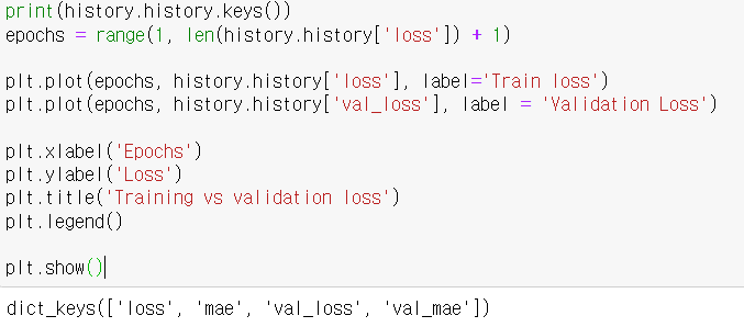
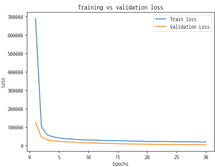
How to Plot Training and Validation Loss
Useful saving tips
🔹 How to Save a Dictionary as a CSV File
A dictionary can be converted into a Pandas DataFrame and then saved as a CSV file.
import pandas as pd

# Example dictionary
data = {
    "Name": ["Alice", "Bob", "Charlie"],
    "Age": [25, 30, 35],
    "City": ["New York", "San Francisco", "Los Angeles"]
}

# Convert dictionary to DataFrame
df = pd.DataFrame(data)

# Save DataFrame as CSV
df.to_csv("output.csv", index=False)  # index=False prevents saving row numbers
🔹 Single Line Code to Save a Matplotlib Plot as PNG
plt.savefig("plot.png", dpi=300) # Save current plot as 'plot.png' with high resolutionHere are one-liners to save and load models for both PyTorch and TensorFlow.
🔹 PyTorch
# Save model
torch.save(model.state_dict(), "model.pth")

# Load model
model.load_state_dict(torch.load("model.pth"))
model.eval()  # Set to evaluation mode
🔹 TensorFlow (Keras)
# Save model
model.save("model.h5")

# Load model
model = keras.models.load_model("model.h5")