CH7-04 Credit Card Fraud Detection 데이터셋 분석
import pandas as pd
import numpy as np
import matplotlib.pyplot as plt
import seaborn as sns
import koreanize_matplotlib
from sklearn.metrics import accuracy_score, f1_score, recall_score, precision_score, roc_curve, roc_auc_score
from sklearn.model_selection import train_test_split
from sklearn.preprocessing import StandardScaler
from sklearn.linear_model import LogisticRegression
from sklearn.ensemble import RandomForestClassifier
from xgboost import XGBClassifier
from lightgbm import LGBMClassifier
raw_df = pd.read_csv('../datas/creditcard.csv')
raw_df| Time | V1 | V2 | V3 | V4 | V5 | V6 | V7 | V8 | V9 | ... | V21 | V22 | V23 | V24 | V25 | V26 | V27 | V28 | Amount | Class | |
|---|---|---|---|---|---|---|---|---|---|---|---|---|---|---|---|---|---|---|---|---|---|
| 0 | 0.0 | -1.359807 | -0.072781 | 2.536347 | 1.378155 | -0.338321 | 0.462388 | 0.239599 | 0.098698 | 0.363787 | ... | -0.018307 | 0.277838 | -0.110474 | 0.066928 | 0.128539 | -0.189115 | 0.133558 | -0.021053 | 149.62 | 0 |
| 1 | 0.0 | 1.191857 | 0.266151 | 0.166480 | 0.448154 | 0.060018 | -0.082361 | -0.078803 | 0.085102 | -0.255425 | ... | -0.225775 | -0.638672 | 0.101288 | -0.339846 | 0.167170 | 0.125895 | -0.008983 | 0.014724 | 2.69 | 0 |
| 2 | 1.0 | -1.358354 | -1.340163 | 1.773209 | 0.379780 | -0.503198 | 1.800499 | 0.791461 | 0.247676 | -1.514654 | ... | 0.247998 | 0.771679 | 0.909412 | -0.689281 | -0.327642 | -0.139097 | -0.055353 | -0.059752 | 378.66 | 0 |
| 3 | 1.0 | -0.966272 | -0.185226 | 1.792993 | -0.863291 | -0.010309 | 1.247203 | 0.237609 | 0.377436 | -1.387024 | ... | -0.108300 | 0.005274 | -0.190321 | -1.175575 | 0.647376 | -0.221929 | 0.062723 | 0.061458 | 123.50 | 0 |
| 4 | 2.0 | -1.158233 | 0.877737 | 1.548718 | 0.403034 | -0.407193 | 0.095921 | 0.592941 | -0.270533 | 0.817739 | ... | -0.009431 | 0.798278 | -0.137458 | 0.141267 | -0.206010 | 0.502292 | 0.219422 | 0.215153 | 69.99 | 0 |
| ... | ... | ... | ... | ... | ... | ... | ... | ... | ... | ... | ... | ... | ... | ... | ... | ... | ... | ... | ... | ... | ... |
| 284802 | 172786.0 | -11.881118 | 10.071785 | -9.834783 | -2.066656 | -5.364473 | -2.606837 | -4.918215 | 7.305334 | 1.914428 | ... | 0.213454 | 0.111864 | 1.014480 | -0.509348 | 1.436807 | 0.250034 | 0.943651 | 0.823731 | 0.77 | 0 |
| 284803 | 172787.0 | -0.732789 | -0.055080 | 2.035030 | -0.738589 | 0.868229 | 1.058415 | 0.024330 | 0.294869 | 0.584800 | ... | 0.214205 | 0.924384 | 0.012463 | -1.016226 | -0.606624 | -0.395255 | 0.068472 | -0.053527 | 24.79 | 0 |
| 284804 | 172788.0 | 1.919565 | -0.301254 | -3.249640 | -0.557828 | 2.630515 | 3.031260 | -0.296827 | 0.708417 | 0.432454 | ... | 0.232045 | 0.578229 | -0.037501 | 0.640134 | 0.265745 | -0.087371 | 0.004455 | -0.026561 | 67.88 | 0 |
| 284805 | 172788.0 | -0.240440 | 0.530483 | 0.702510 | 0.689799 | -0.377961 | 0.623708 | -0.686180 | 0.679145 | 0.392087 | ... | 0.265245 | 0.800049 | -0.163298 | 0.123205 | -0.569159 | 0.546668 | 0.108821 | 0.104533 | 10.00 | 0 |
| 284806 | 172792.0 | -0.533413 | -0.189733 | 0.703337 | -0.506271 | -0.012546 | -0.649617 | 1.577006 | -0.414650 | 0.486180 | ... | 0.261057 | 0.643078 | 0.376777 | 0.008797 | -0.473649 | -0.818267 | -0.002415 | 0.013649 | 217.00 | 0 |
284807 rows × 31 columns
raw_df.info()<class 'pandas.core.frame.DataFrame'>
RangeIndex: 284807 entries, 0 to 284806
Data columns (total 31 columns):
# Column Non-Null Count Dtype
--- ------ -------------- -----
0 Time 284807 non-null float64
1 V1 284807 non-null float64
2 V2 284807 non-null float64
3 V3 284807 non-null float64
4 V4 284807 non-null float64
5 V5 284807 non-null float64
6 V6 284807 non-null float64
7 V7 284807 non-null float64
8 V8 284807 non-null float64
9 V9 284807 non-null float64
10 V10 284807 non-null float64
11 V11 284807 non-null float64
12 V12 284807 non-null float64
13 V13 284807 non-null float64
14 V14 284807 non-null float64
15 V15 284807 non-null float64
16 V16 284807 non-null float64
17 V17 284807 non-null float64
18 V18 284807 non-null float64
19 V19 284807 non-null float64
20 V20 284807 non-null float64
21 V21 284807 non-null float64
22 V22 284807 non-null float64
23 V23 284807 non-null float64
24 V24 284807 non-null float64
25 V25 284807 non-null float64
26 V26 284807 non-null float64
27 V27 284807 non-null float64
28 V28 284807 non-null float64
29 Amount 284807 non-null float64
30 Class 284807 non-null int64
dtypes: float64(30), int64(1)
memory usage: 67.4 MB1. 칼럼 명세
- V1~V28은 개인정보보호를 이유로 PCA로 차원축소된 개인정보 피처들임
- Amount는 거래량
- Class 1은 Fraud, 0은 Not Fraud
2. 4개 모델 한꺼번에 훈련하는 함수, [f1,precision,accuracy,recall] 스코어 함수, 그 점수를 데이터프레임으로 모델이름, 점수 담는 함수 만들기
def scores(pred, y_test):
f1 = f1_score(y_test, pred)
acc = accuracy_score(y_test, pred)
precision = precision_score(y_test, pred)
rec = recall_score(y_test, pred)
roc_score = roc_auc_score(y_test, pred)
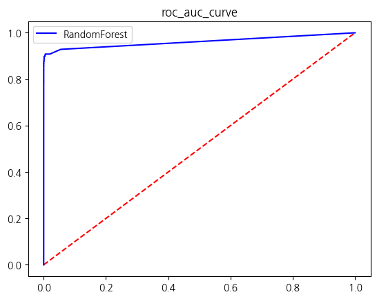
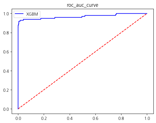
return acc, precision, rec, f1, roc_scoredef train_models(model, X_train, y_train, X_test, y_test):
model.fit(X_train, y_train)
pred = model.predict(X_test)
proba = model.predict_proba(X_test)
return scores(pred, y_test), probadef get_score_df(models, X_train, y_train, X_test, y_test):
tmp = []
names = ['LogisticRegression', 'RandomForest', 'XGBM', 'LGBM']
for model,name in zip(models, names):
score, proba = train_models(model, X_train, y_train, X_test, y_test)
tmp.append(pd.DataFrame({'accuracy':score[0],
'precision':score[1],
'recall':score[2],
'f1_score':score[3],
'roc_auc_score':score[4]},index = [name]))
fpr, tpr, thresholds = roc_curve(y_test, proba[:,1])
plt.plot([0,1],[0,1],color = 'red', ls = 'dashed')
plt.plot(fpr, tpr, color = 'blue', label = f'{name}')
plt.legend()
plt.title('roc_auc_curve')
plt.show()
return pd.concat(tmp, axis = 0)3. 클래스 불균형 살펴보기
sns.countplot(raw_df, x = 'Class', hue = 'Class')<Axes: xlabel='Class', ylabel='count'>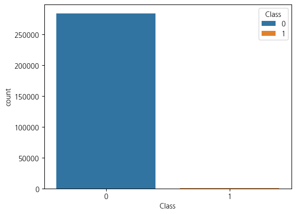
raw_df.describe()| Time | V1 | V2 | V3 | V4 | V5 | V6 | V7 | V8 | V9 | ... | V21 | V22 | V23 | V24 | V25 | V26 | V27 | V28 | Amount | Class | |
|---|---|---|---|---|---|---|---|---|---|---|---|---|---|---|---|---|---|---|---|---|---|
| count | 284807.000000 | 2.848070e+05 | 2.848070e+05 | 2.848070e+05 | 2.848070e+05 | 2.848070e+05 | 2.848070e+05 | 2.848070e+05 | 2.848070e+05 | 2.848070e+05 | ... | 2.848070e+05 | 2.848070e+05 | 2.848070e+05 | 2.848070e+05 | 2.848070e+05 | 2.848070e+05 | 2.848070e+05 | 2.848070e+05 | 284807.000000 | 284807.000000 |
| mean | 94813.859575 | 1.168375e-15 | 3.416908e-16 | -1.379537e-15 | 2.074095e-15 | 9.604066e-16 | 1.487313e-15 | -5.556467e-16 | 1.213481e-16 | -2.406331e-15 | ... | 1.654067e-16 | -3.568593e-16 | 2.578648e-16 | 4.473266e-15 | 5.340915e-16 | 1.683437e-15 | -3.660091e-16 | -1.227390e-16 | 88.349619 | 0.001727 |
| std | 47488.145955 | 1.958696e+00 | 1.651309e+00 | 1.516255e+00 | 1.415869e+00 | 1.380247e+00 | 1.332271e+00 | 1.237094e+00 | 1.194353e+00 | 1.098632e+00 | ... | 7.345240e-01 | 7.257016e-01 | 6.244603e-01 | 6.056471e-01 | 5.212781e-01 | 4.822270e-01 | 4.036325e-01 | 3.300833e-01 | 250.120109 | 0.041527 |
| min | 0.000000 | -5.640751e+01 | -7.271573e+01 | -4.832559e+01 | -5.683171e+00 | -1.137433e+02 | -2.616051e+01 | -4.355724e+01 | -7.321672e+01 | -1.343407e+01 | ... | -3.483038e+01 | -1.093314e+01 | -4.480774e+01 | -2.836627e+00 | -1.029540e+01 | -2.604551e+00 | -2.256568e+01 | -1.543008e+01 | 0.000000 | 0.000000 |
| 25% | 54201.500000 | -9.203734e-01 | -5.985499e-01 | -8.903648e-01 | -8.486401e-01 | -6.915971e-01 | -7.682956e-01 | -5.540759e-01 | -2.086297e-01 | -6.430976e-01 | ... | -2.283949e-01 | -5.423504e-01 | -1.618463e-01 | -3.545861e-01 | -3.171451e-01 | -3.269839e-01 | -7.083953e-02 | -5.295979e-02 | 5.600000 | 0.000000 |
| 50% | 84692.000000 | 1.810880e-02 | 6.548556e-02 | 1.798463e-01 | -1.984653e-02 | -5.433583e-02 | -2.741871e-01 | 4.010308e-02 | 2.235804e-02 | -5.142873e-02 | ... | -2.945017e-02 | 6.781943e-03 | -1.119293e-02 | 4.097606e-02 | 1.659350e-02 | -5.213911e-02 | 1.342146e-03 | 1.124383e-02 | 22.000000 | 0.000000 |
| 75% | 139320.500000 | 1.315642e+00 | 8.037239e-01 | 1.027196e+00 | 7.433413e-01 | 6.119264e-01 | 3.985649e-01 | 5.704361e-01 | 3.273459e-01 | 5.971390e-01 | ... | 1.863772e-01 | 5.285536e-01 | 1.476421e-01 | 4.395266e-01 | 3.507156e-01 | 2.409522e-01 | 9.104512e-02 | 7.827995e-02 | 77.165000 | 0.000000 |
| max | 172792.000000 | 2.454930e+00 | 2.205773e+01 | 9.382558e+00 | 1.687534e+01 | 3.480167e+01 | 7.330163e+01 | 1.205895e+02 | 2.000721e+01 | 1.559499e+01 | ... | 2.720284e+01 | 1.050309e+01 | 2.252841e+01 | 4.584549e+00 | 7.519589e+00 | 3.517346e+00 | 3.161220e+01 | 3.384781e+01 | 25691.160000 | 1.000000 |
8 rows × 31 columns
4. 클래스의 비율 value_counts(normalize=True)로 확인하기
- Fraud인 클래스 1의 비율이 전체에서 0.1727%로 굉장히 심하게 불균형한 데이터임
raw_df['Class'].value_counts(normalize=True)Class
0 0.998273
1 0.001727
Name: proportion, dtype: float645. 일단 아무런 전처리 없이 모델 돌려보기
X = raw_df.drop(['Time','Class'], axis = 1)
y = raw_df['Class']X_train, X_test, y_train, y_test = train_test_split(X, y, stratify = y, test_size = 0.2, random_state = 42)lr_clf = LogisticRegression(n_jobs = -1, random_state = 42, solver = 'liblinear')
rf_clf = RandomForestClassifier(n_estimators = 300, oob_score = True, n_jobs = -1, random_state = 42)
XGB_clf = XGBClassifier(n_jobs = -1, random_state = 42, verbosity = 1, n_estimators = 100)
LGBM_clf = LGBMClassifier(n_jobs = -1, random_state = 42, verbosity = 1, n_estimators = 1000,num_leaves = 186, learning_rate=0.15, boost_from_average = False)models = [lr_clf, rf_clf, XGB_clf, LGBM_clf]res = get_score_df(models, X_train, y_train, X_test, y_test)C:\Users\kd010\miniconda3\Lib\site-packages\sklearn\linear_model\_logistic.py:1222: UserWarning: 'n_jobs' > 1 does not have any effect when 'solver' is set to 'liblinear'. Got 'n_jobs' = 16.
warnings.warn(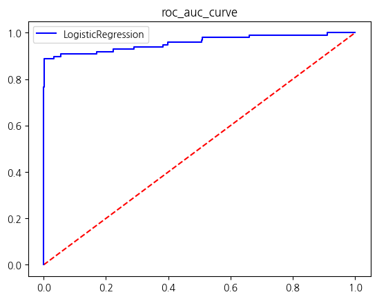
[LightGBM] [Info] Number of positive: 394, number of negative: 227451
[LightGBM] [Info] Auto-choosing col-wise multi-threading, the overhead of testing was 0.009062 seconds.
You can set `force_col_wise=true` to remove the overhead.
[LightGBM] [Info] Total Bins 7395
[LightGBM] [Info] Number of data points in the train set: 227845, number of used features: 29
[LightGBM] [Warning] No further splits with positive gain, best gain: -inf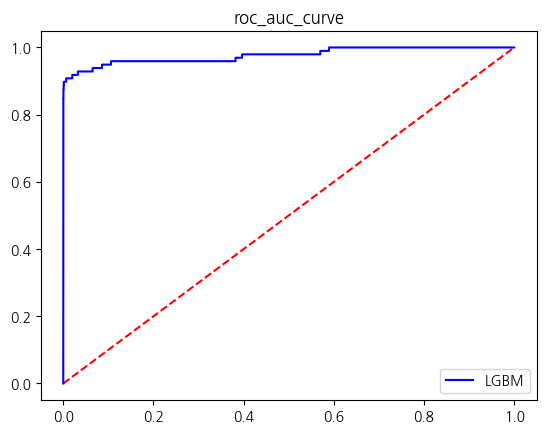
res| accuracy | precision | recall | f1_score | roc_auc_score | |
|---|---|---|---|---|---|
| LogisticRegression | 0.999157 | 0.828947 | 0.642857 | 0.724138 | 0.821314 |
| RandomForest | 0.999596 | 0.941176 | 0.816327 | 0.874317 | 0.908119 |
| XGBM | 0.999561 | 0.919540 | 0.816327 | 0.864865 | 0.908102 |
| LGBM | 0.999561 | 0.929412 | 0.806122 | 0.863388 | 0.903008 |