6. amount 피처에 StandardScaler적용시켜보기(recall이 오히려 떨어졌다 precision은 약간 증가, f1은 감소, roc_auc도 감소)
scaler = StandardScaler()
amount_sc = scaler.fit_transform(np.array(X['Amount']).reshape(-1,1))
X_copy = X.iloc[:,:-1].copy()
X_copy['Amount_scaled'] = amount_scX_copy_train, X_copy_test, y_train, y_test = train_test_split(X_copy, y,random_state = 42, test_size = 0.3, stratify = y)get_score_df(models, X_copy_train, y_train, X_copy_test, y_test)C:\Users\kd010\miniconda3\Lib\site-packages\sklearn\linear_model\_logistic.py:1222: UserWarning: 'n_jobs' > 1 does not have any effect when 'solver' is set to 'liblinear'. Got 'n_jobs' = 16.
warnings.warn(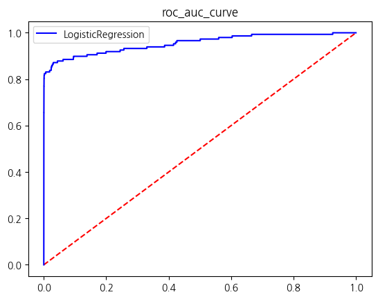

[LightGBM] [Info] Number of positive: 344, number of negative: 199020
[LightGBM] [Info] Auto-choosing col-wise multi-threading, the overhead of testing was 0.009484 seconds.
You can set `force_col_wise=true` to remove the overhead.
[LightGBM] [Info] Total Bins 7395
[LightGBM] [Info] Number of data points in the train set: 199364, number of used features: 29
[LightGBM] [Warning] No further splits with positive gain, best gain: -inf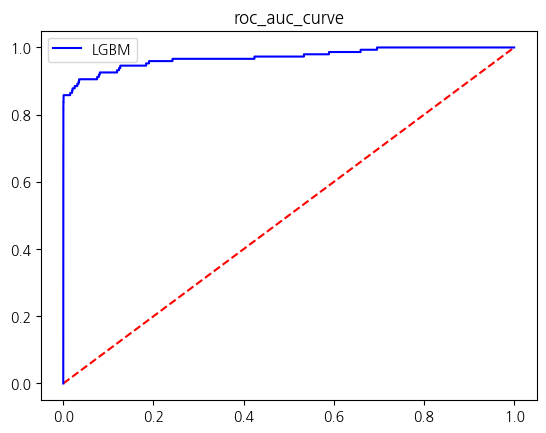
| accuracy | precision | recall | f1_score | roc_auc_score | |
|---|---|---|---|---|---|
| LogisticRegression | 0.999169 | 0.859813 | 0.621622 | 0.721569 | 0.810723 |
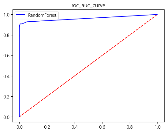
| RandomForest | 0.999532 | 0.957627 | 0.763514 | 0.849624 | 0.881727 |
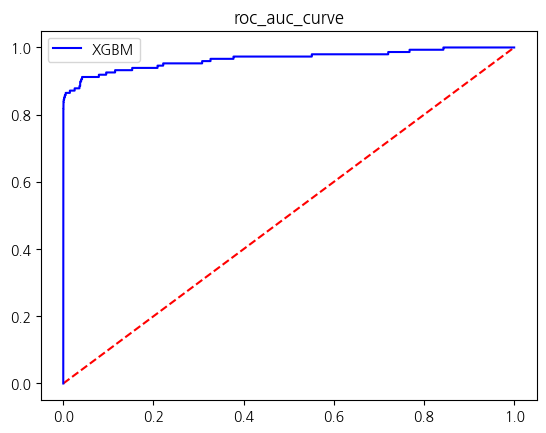
| XGBM | 0.999520 | 0.942149 | 0.770270 | 0.847584 | 0.885094 |
| LGBM | 0.999508 | 0.941667 | 0.763514 | 0.843284 | 0.881716 |
7. amount 피처 로그 변환 해보기 lop1p() = log(1+x) 활용
- LogisticRegression의 recall이 약간 증가한것 0.01정도 빼고는 별 변화 없음
- 로그 변환 결과 분포가 훨씬 균일해짐
X_log = X.iloc[:,:-1].copy()
amount_log = np.log1p(np.array(X['Amount']).reshape(-1,1))X_log['Amount_log'] = amount_logX_log_train, X_log_test, y_train, y_test = train_test_split(X_log, y, stratify = y, random_state = 42, test_size = 0.2)get_score_df(models, X_log_train, y_train, X_log_test, y_test)C:\Users\kd010\miniconda3\Lib\site-packages\sklearn\linear_model\_logistic.py:1222: UserWarning: 'n_jobs' > 1 does not have any effect when 'solver' is set to 'liblinear'. Got 'n_jobs' = 16.
warnings.warn(
[LightGBM] [Info] Number of positive: 394, number of negative: 227451
[LightGBM] [Info] Auto-choosing col-wise multi-threading, the overhead of testing was 0.009853 seconds.
You can set `force_col_wise=true` to remove the overhead.
[LightGBM] [Info] Total Bins 7395
[LightGBM] [Info] Number of data points in the train set: 227845, number of used features: 29
[LightGBM] [Warning] No further splits with positive gain, best gain: -inf
| accuracy | precision | recall | f1_score | roc_auc_score | |
|---|---|---|---|---|---|
| LogisticRegression | 0.999175 | 0.831169 | 0.653061 | 0.731429 | 0.826416 |
| RandomForest | 0.999596 | 0.941176 | 0.816327 | 0.874317 | 0.908119 |
| XGBM | 0.999561 | 0.919540 | 0.816327 | 0.864865 | 0.908102 |
| LGBM | 0.999561 | 0.929412 | 0.806122 | 0.863388 | 0.903008 |
sns.histplot(X_log, x='Amount_log')<Axes: xlabel='Amount_log', ylabel='Count'>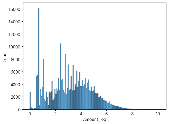
8. 대략 boxplot으로 이상치 파악하기
fig, ax = plt.subplots(2,1,figsize=(12,7))
sns.boxplot(X.iloc[:,:10],ax = ax[0])
sns.boxplot(X.iloc[:,10:-1],ax=ax[1])
plt.show()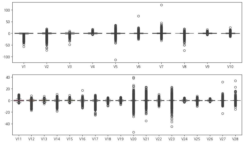
9. V20, V21, V23의 이상치가 많아보이므로 이상치 없애보기
def set_outliers(data, column):

    fraud = data[data['Class'] == 0][column]
    q1 = np.quantile(fraud, 0.25)
    q3 = np.quantile(fraud, 0.75)

    iqr = q3 - q1
    lower_bound = q1 - 1.5*iqr
    upper_bound = q3 + 1.5*iqr
    cond1 = fraud < lower_bound
    cond2 = fraud > upper_bound
    indexes = fraud[cond1 | cond2].index

    return indexes.tolist()
X_cols = X.columns.tolist()outliers_indexes = []
for col in ['V20','V21','V23']:
outliers_indexes.extend(set_outliers(raw_df, col))outliers = list(set([i for i in outliers_indexes[::1]]))print(len(outliers))38892new_df = raw_df.drop(index=outliers)new_df| Time | V1 | V2 | V3 | V4 | V5 | V6 | V7 | V8 | V9 | ... | V21 | V22 | V23 | V24 | V25 | V26 | V27 | V28 | Amount | Class | |
|---|---|---|---|---|---|---|---|---|---|---|---|---|---|---|---|---|---|---|---|---|---|
| 0 | 0.0 | -1.359807 | -0.072781 | 2.536347 | 1.378155 | -0.338321 | 0.462388 | 0.239599 | 0.098698 | 0.363787 | ... | -0.018307 | 0.277838 | -0.110474 | 0.066928 | 0.128539 | -0.189115 | 0.133558 | -0.021053 | 149.62 | 0 |
| 1 | 0.0 | 1.191857 | 0.266151 | 0.166480 | 0.448154 | 0.060018 | -0.082361 | -0.078803 | 0.085102 | -0.255425 | ... | -0.225775 | -0.638672 | 0.101288 | -0.339846 | 0.167170 | 0.125895 | -0.008983 | 0.014724 | 2.69 | 0 |
| 3 | 1.0 | -0.966272 | -0.185226 | 1.792993 | -0.863291 | -0.010309 | 1.247203 | 0.237609 | 0.377436 | -1.387024 | ... | -0.108300 | 0.005274 | -0.190321 | -1.175575 | 0.647376 | -0.221929 | 0.062723 | 0.061458 | 123.50 | 0 |
| 4 | 2.0 | -1.158233 | 0.877737 | 1.548718 | 0.403034 | -0.407193 | 0.095921 | 0.592941 | -0.270533 | 0.817739 | ... | -0.009431 | 0.798278 | -0.137458 | 0.141267 | -0.206010 | 0.502292 | 0.219422 | 0.215153 | 69.99 | 0 |
| 5 | 2.0 | -0.425966 | 0.960523 | 1.141109 | -0.168252 | 0.420987 | -0.029728 | 0.476201 | 0.260314 | -0.568671 | ... | -0.208254 | -0.559825 | -0.026398 | -0.371427 | -0.232794 | 0.105915 | 0.253844 | 0.081080 | 3.67 | 0 |
| ... | ... | ... | ... | ... | ... | ... | ... | ... | ... | ... | ... | ... | ... | ... | ... | ... | ... | ... | ... | ... | ... |
| 284801 | 172785.0 | 0.120316 | 0.931005 | -0.546012 | -0.745097 | 1.130314 | -0.235973 | 0.812722 | 0.115093 | -0.204064 | ... | -0.314205 | -0.808520 | 0.050343 | 0.102800 | -0.435870 | 0.124079 | 0.217940 | 0.068803 | 2.69 | 0 |
| 284803 | 172787.0 | -0.732789 | -0.055080 | 2.035030 | -0.738589 | 0.868229 | 1.058415 | 0.024330 | 0.294869 | 0.584800 | ... | 0.214205 | 0.924384 | 0.012463 | -1.016226 | -0.606624 | -0.395255 | 0.068472 | -0.053527 | 24.79 | 0 |
| 284804 | 172788.0 | 1.919565 | -0.301254 | -3.249640 | -0.557828 | 2.630515 | 3.031260 | -0.296827 | 0.708417 | 0.432454 | ... | 0.232045 | 0.578229 | -0.037501 | 0.640134 | 0.265745 | -0.087371 | 0.004455 | -0.026561 | 67.88 | 0 |
| 284805 | 172788.0 | -0.240440 | 0.530483 | 0.702510 | 0.689799 | -0.377961 | 0.623708 | -0.686180 | 0.679145 | 0.392087 | ... | 0.265245 | 0.800049 | -0.163298 | 0.123205 | -0.569159 | 0.546668 | 0.108821 | 0.104533 | 10.00 | 0 |
| 284806 | 172792.0 | -0.533413 | -0.189733 | 0.703337 | -0.506271 | -0.012546 | -0.649617 | 1.577006 | -0.414650 | 0.486180 | ... | 0.261057 | 0.643078 | 0.376777 | 0.008797 | -0.473649 | -0.818267 | -0.002415 | 0.013649 | 217.00 | 0 |
245915 rows × 31 columns
10. Class가 0인 것(Not Fraud) 중 V20, V21, V23칼럼의 이상치 제거만 하고 성능평가하기
- 나의 논리는 Not Fraud로 라벨링 된 것 중 이상치들은 사실 Fraud로 분류되어야 하지 않았을까 라는 생각에서 V20, V21, V23의 oulier를 iqr에 기반하여 제거하였다
- 제거한 후 성능을 보면 현재까지 시도(raw데이터, amount칼럼 standardscaling, amount칼럼 log변환)중 가장 높은 recall과 precision, f1score 모두 압도적으로 높다
X = new_df.drop(['Time','Class'],axis=1)
y = new_df['Class']X_train, X_test, y_train, y_test = train_test_split(X, y, test_size = 0.2, stratify = y, random_state = 42)get_score_df(models, X_train, y_train, X_test, y_test)

[LightGBM] [Info] Number of positive: 394, number of negative: 196338
[LightGBM] [Info] Auto-choosing col-wise multi-threading, the overhead of testing was 0.007124 seconds.
You can set `force_col_wise=true` to remove the overhead.
[LightGBM] [Info] Total Bins 7395
[LightGBM] [Info] Number of data points in the train set: 196732, number of used features: 29
[LightGBM] [Warning] No further splits with positive gain, best gain: -inf
| accuracy | precision | recall | f1_score | roc_auc_score | |
|---|---|---|---|---|---|
| LogisticRegression | 0.999614 | 0.975904 | 0.826531 | 0.895028 | 0.913245 |
| RandomForest | 0.999634 | 0.965116 | 0.846939 | 0.902174 | 0.923439 |
| XGBM | 0.999675 | 0.988095 | 0.846939 | 0.912088 | 0.923459 |
| LGBM | 0.999654 | 1.000000 | 0.826531 | 0.905028 | 0.913265 |
11. Outlier 제거된 데이터에서 Amount열을 log변환 한 성능 평가
- V20, V21, V23 열 중에 Class가 0인것 중 iqr을 기준으로 outlier를 제거한 것과 그 데이터를 기반으로 Amount칼럼을 log변환한 성능이 동일함
X_log = X.iloc[:,:-1].copy()
amount_log = np.log1p(X['Amount'])
X_log['Amount_log'] = amount_logX_log_train, X_log_test, y_train, y_test = train_test_split(X_log, y, test_size=0.2, random_state=42, stratify=y)get_score_df(models, X_log_train, y_train, X_log_test, y_test)


[LightGBM] [Info] Number of positive: 394, number of negative: 196338
[LightGBM] [Info] Auto-choosing col-wise multi-threading, the overhead of testing was 0.007568 seconds.
You can set `force_col_wise=true` to remove the overhead.
[LightGBM] [Info] Total Bins 7395
[LightGBM] [Info] Number of data points in the train set: 196732, number of used features: 29
[LightGBM] [Warning] No further splits with positive gain, best gain: -inf

| accuracy | precision | recall | f1_score | roc_auc_score | |
|---|---|---|---|---|---|
| LogisticRegression | 0.999614 | 0.975904 | 0.826531 | 0.895028 | 0.913245 |
| RandomForest | 0.999634 | 0.965116 | 0.846939 | 0.902174 | 0.923439 |
| XGBM | 0.999675 | 0.988095 | 0.846939 | 0.912088 | 0.923459 |
| LGBM | 0.999654 | 1.000000 | 0.826531 | 0.905028 | 0.913265 |