CH6-03. 앙상블 기법
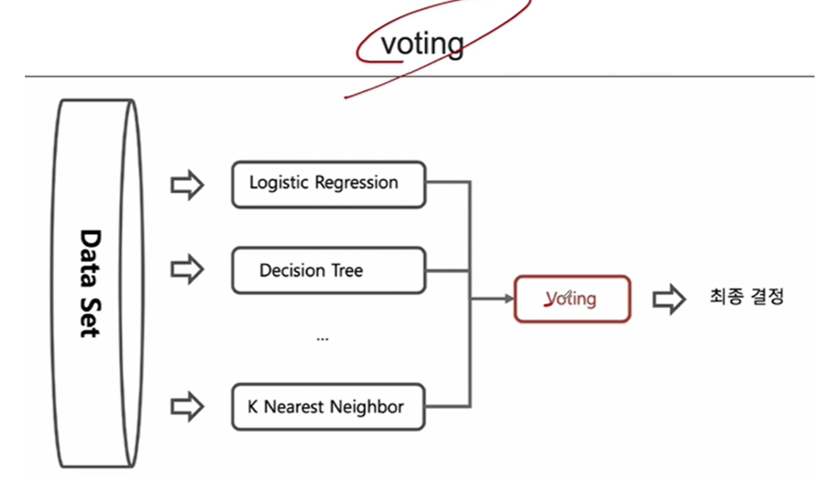
1. 앙상블 기법 중 (Voting 기법)
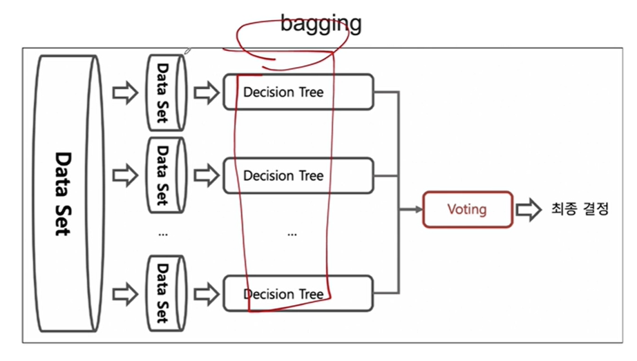
2. 배깅(Bootstrap Aggregation)
- 중복을 허용하여 랜덤 샘플링하는 부트스트랩을 각 약분류기에 적용한다.
- 랜덤 포레스트에서 쓰이는 기법이다.
- 각 약분류기에 쓰이는 모델은 동일하다 .
- 랜덤 포레스트는 정형데이터에 굉장히 강력하며 속도도 빠르고 성능도 좋다
- 최종 결정은 소프트보팅을 쓰게 된다.
- 랜덤 포레스트에서 회귀와 분류에 적용되는 보팅 방식
-
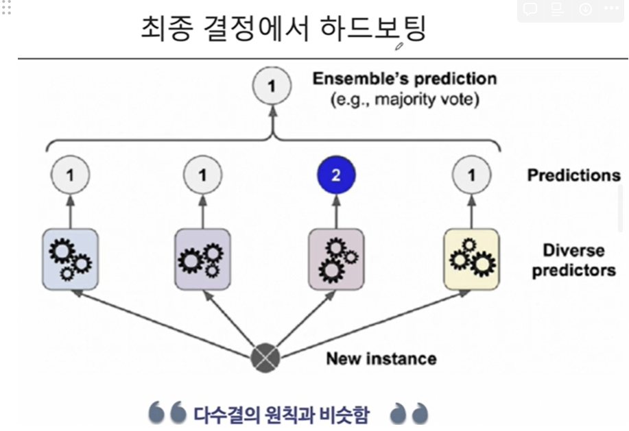
다수결 투표(Majority Voting): 분류(Classification) 문제에서, 각 결정 트리가 하나의 클래스를 예측하고, 가장 많이 예측된 클래스가 최종 결과가 됩니다. 이 방식은 소프트 보팅과 다른, 하드 보팅(Hard Voting)의 한 예입니다.
-
평균(Averaging): 회귀(Regression) 문제에서, 각 결정 트리의 예측값의 평균을 내어 최종 예측값을 결정합니다.
소프트 보팅(Soft Voting)은 각 클래스에 대한 예측 확률을 평균내어, 가장 높은 확률을 가진 클래스를 최종 예측값으로 결정하는 방식입니다. 이 방법은 각 모델이 클래스의 소속 확률을 제공할 수 있을 때 사용됩니다. 랜덤 포레스트는 기본적으로 하드 보팅 방식을 사용하지만, 각 결정 트리의 예측 확률을 평균내어 소프트 보팅과 유사한 방식으로 활용할 수 있습니다. 즉, 분류 문제에서 랜덤 포레스트 모델이 각 클래스에 대한 확률을 출력하도록 할 수 있으며, 이를 바탕으로 더 정교한 결정을 내릴 수 있습니다.
따라서, 랜덤 포레스트는 기본적으로는 하드 보팅 방식을 사용하지만, 필요에 따라 소프트 보팅 방식을 사용할 수 있는 유연성을 가지고 있습니다.
-
3. 결정 과정에서의 하드보팅(다수결)
4. 결정 과정에서의 소프트보팅(확률의 평균)

- 여기서 클래스 1로 예측한게 3개임(0.9 + 0.8 + 0.4)/3 = 0.7
- 여기서 클래스 2로 예측한게 1개(0.7))
- 두 클래스의 확률이 0.7로 동률이므로 하드보팅으로 1로 결정됨
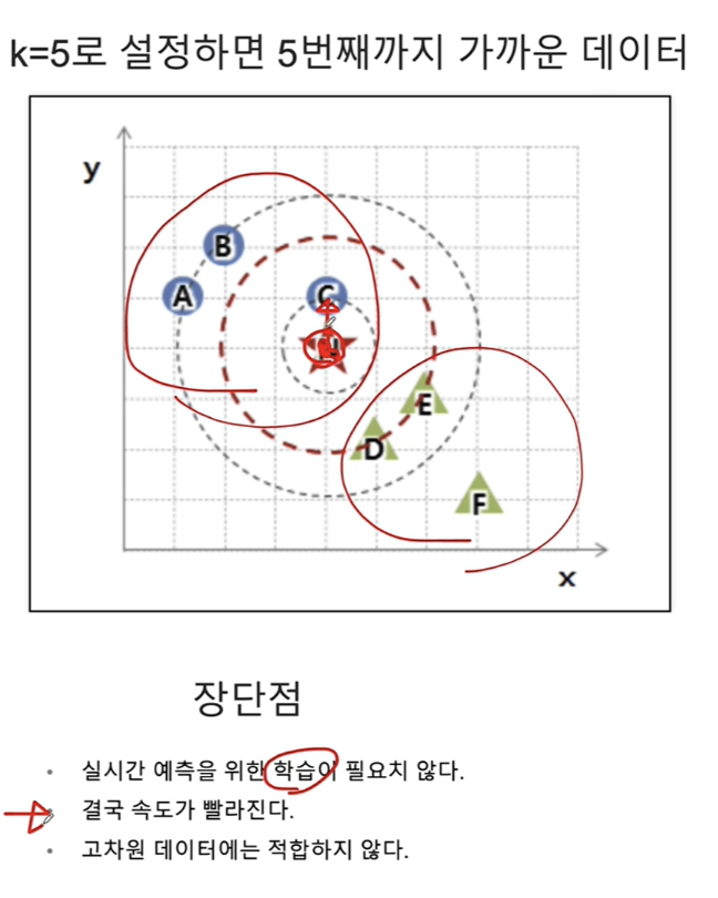
CH7-02 KNN
네, K-최근접 이웃(K-Nearest Neighbors, KNN) 알고리즘은 주어진 데이터 포인트에 대해 가장 가까운 (k)개의 이웃 데이터 포인트를 찾고, 이 이웃들이 가장 많이 속한 라벨(클래스)로 데이터 포인트를 분류합니다. (k)값은 사용자가 지정하는 하이퍼파라미터이며, 이 값에 따라 모델의 분류 성능이 달라질 수 있습니다.
KNN 분류 과정은 다음과 같습니다:
- 거리 측정: 데이터 포인트 간의 거리를 측정하기 위한 방법을 선택합니다. 일반적으로 유클리디안 거리가 사용되지만, 맨해튼 거리나 민코프스키 거리와 같은 다른 거리 측정 방법도 사용될 수 있습니다.
- 최근접 이웃 찾기: 분류하고자 하는 데이터 포인트로부터 가장 가까운 (k)개의 이웃을 찾습니다.
- 다수결 투표: 찾아낸 (k)개의 이웃 중 가장 많이 속한 라벨로 데이터 포인트를 분류합니다. 각 이웃은 동일한 가중치를 가지고 투표할 수 있으며, 이를 '단순 다수결 투표'라고 합니다. 또한, 이웃의 거리에 따라 가중치를 다르게 주어 투표할 수도 있으며, 이 경우 거리가 가까울수록 더 큰 영향을 미치게 됩니다.
(k)값의 선택은 매우 중요합니다. (k)값이 너무 작으면 노이즈에 민감해져 과적합(overfitting)이 발생할 수 있고, (k)값이 너무 크면 모델이 과도하게 일반화되어 과소적합(underfitting)이 발생할 수 있습니다. 따라서 적절한 (k)값을 찾기 위해 교차 검증과 같은 방법을 사용하는 것이 좋습니다.
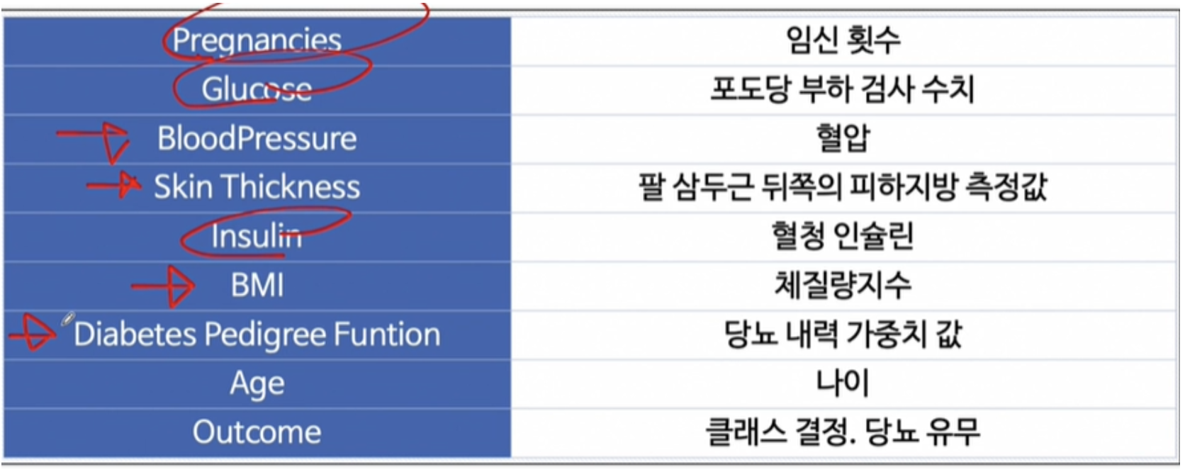
CH.6-03 PIMA 인디언 당뇨병 예측
df.info()<class 'pandas.core.frame.DataFrame'>
RangeIndex: 768 entries, 0 to 767
Data columns (total 9 columns):
# Column Non-Null Count Dtype
--- ------ -------------- -----
0 Pregnancies 768 non-null int64
1 Glucose 768 non-null int64
2 BloodPressure 768 non-null int64
3 SkinThickness 768 non-null int64
4 Insulin 768 non-null int64
5 BMI 768 non-null float64
6 DiabetesPedigreeFunction 768 non-null float64
7 Age 768 non-null int64
8 Outcome 768 non-null int64
dtypes: float64(2), int64(7)
memory usage: 54.1 KB1. 칼럼 명세
df.describe()| Pregnancies | Glucose | BloodPressure | SkinThickness | Insulin | BMI | DiabetesPedigreeFunction | Age | Outcome | |
|---|---|---|---|---|---|---|---|---|---|
| count | 768.000000 | 768.000000 | 768.000000 | 768.000000 | 768.000000 | 768.000000 | 768.000000 | 768.000000 | 768.000000 |
| mean | 3.845052 | 120.894531 | 69.105469 | 20.536458 | 79.799479 | 31.992578 | 0.471876 | 33.240885 | 0.348958 |
| std | 3.369578 | 31.972618 | 19.355807 | 15.952218 | 115.244002 | 7.884160 | 0.331329 | 11.760232 | 0.476951 |
| min | 0.000000 | 0.000000 | 0.000000 | 0.000000 | 0.000000 | 0.000000 | 0.078000 | 21.000000 | 0.000000 |
| 25% | 1.000000 | 99.000000 | 62.000000 | 0.000000 | 0.000000 | 27.300000 | 0.243750 | 24.000000 | 0.000000 |
| 50% | 3.000000 | 117.000000 | 72.000000 | 23.000000 | 30.500000 | 32.000000 | 0.372500 | 29.000000 | 0.000000 |
| 75% | 6.000000 | 140.250000 | 80.000000 | 32.000000 | 127.250000 | 36.600000 | 0.626250 | 41.000000 | 1.000000 |
| max | 17.000000 | 199.000000 | 122.000000 | 99.000000 | 846.000000 | 67.100000 | 2.420000 | 81.000000 | 1.000000 |
2. 상관관계 히트맵
corr_mat = df.corr(method = 'pearson')
plt.figure(figsize=(10,10))
sns.heatmap(corr_mat, annot = True, cmap = 'YlGnBu')
3. 결측치나 이상치 찾기
sns.histplot(data = df, x='BloodPressure')<Axes: xlabel='BloodPressure', ylabel='Count'>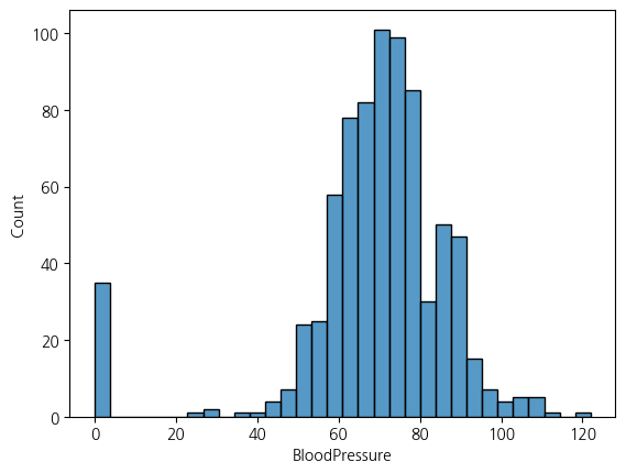
sns.histplot(df, x='Glucose')<Axes: xlabel='Glucose', ylabel='Count'>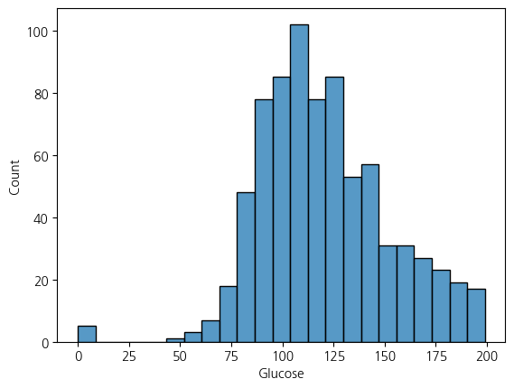
sns.histplot(df, x='SkinThickness', bins=100)<Axes: xlabel='SkinThickness', ylabel='Count'>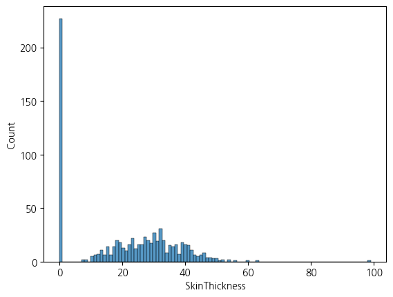
sns.histplot(df, x='Insulin', bins = 300).set_xlim(0,50)(0.0, 50.0)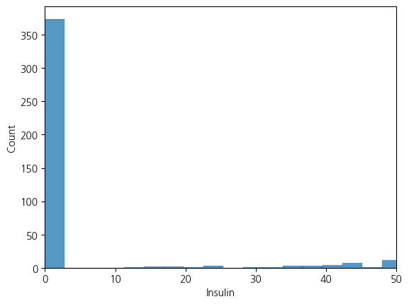
sns.histplot(df, x='BMI')<Axes: xlabel='BMI', ylabel='Count'>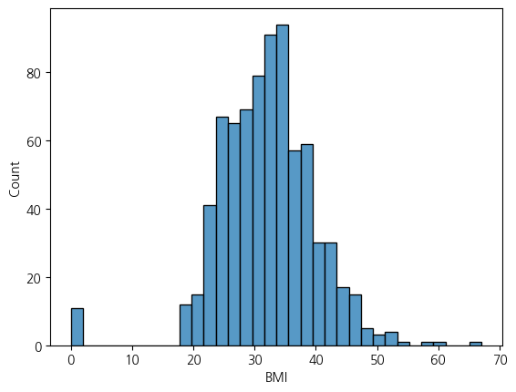
4. 각 피처에서 0인 값들 describe()로 확인하기 Outcome과 Pregnancies는 0이 이상치가 아닐 가능성 높음으로 그냥 놔둠
- 당뇨병 환자의 경우, 특히 제1형 당뇨병 환자에서는 췌장의 인슐린 생산이 심각하게 감소하거나 전혀 이루어지지 않을 수 있습니다. 그러나 실제로 체내 인슐린 수치가 완전히 0이 되는 경우는 극히 드뭅니다. 제1형 당뇨병 환자는 췌장에서 인슐린을 충분히 생산하지 못하기 때문에 외부에서 인슐린을 주입해야 합니다. 이를 통해 혈당 수치를 조절하고 생명을 유지합니다.
제2형 당뇨병 환자의 경우, 췌장이 여전히 인슐린을 생산하지만, 몸이 이를 제대로 사용하지 못하는 상태인 인슐린 저항성 때문에 문제가 발생합니다. 따라서 제2형 당뇨병 환자도 체내 인슐린 수치가 완전히 0이 되는 상황은 일반적이지 않습니다.-
df[df==0].describe()| Pregnancies | Glucose | BloodPressure | SkinThickness | Insulin | BMI | DiabetesPedigreeFunction | Age | Outcome | |
|---|---|---|---|---|---|---|---|---|---|
| count | 111.0 | 5.0 | 35.0 | 227.0 | 374.0 | 11.0 | 0.0 | 0.0 | 500.0 |
| mean | 0.0 | 0.0 | 0.0 | 0.0 | 0.0 | 0.0 | NaN | NaN | 0.0 |
| std | 0.0 | 0.0 | 0.0 | 0.0 | 0.0 | 0.0 | NaN | NaN | 0.0 |
| min | 0.0 | 0.0 | 0.0 | 0.0 | 0.0 | 0.0 | NaN | NaN | 0.0 |
| 25% | 0.0 | 0.0 | 0.0 | 0.0 | 0.0 | 0.0 | NaN | NaN | 0.0 |
| 50% | 0.0 | 0.0 | 0.0 | 0.0 | 0.0 | 0.0 | NaN | NaN | 0.0 |
| 75% | 0.0 | 0.0 | 0.0 | 0.0 | 0.0 | 0.0 | NaN | NaN | 0.0 |
| max | 0.0 | 0.0 | 0.0 | 0.0 | 0.0 | 0.0 | NaN | NaN | 0.0 |
5. Glucose 수치가 0인 데이터를 Outcome에 따라 나누고 평균으로 대체하기
cond1 = (df['Glucose'] == 0) & (df['Outcome'] == 1)
cond2 = (df['Glucose'] == 0) & (df['Outcome'] == 0)
cond3 = (df['Outcome'] == 1)
cond4 = (df['Outcome'] == 0)
df.loc[cond1,'Glucose'] = df.loc[cond3,'Glucose'].mean()
df.loc[cond2,'Glucose'] = df.loc[cond4,'Glucose'].mean()
C:\Users\kd010\AppData\Local\Temp\ipykernel_28296\1895424279.py:5: FutureWarning: Setting an item of incompatible dtype is deprecated and will raise in a future error of pandas. Value '141.25746268656715' has dtype incompatible with int64, please explicitly cast to a compatible dtype first.
df.loc[cond1,'Glucose'] = df.loc[cond3,'Glucose'].mean()df.Glucose.describe()count 768.000000
mean 121.691999
std 30.461151
min 44.000000
25% 99.750000
50% 117.000000
75% 141.000000
max 199.000000
Name: Glucose, dtype: float646. BloodPressure 0값들 채우기
cond1 = df['BloodPressure'] == 0
cond2 = df['Outcome'] == 0

df.loc[cond1 & cond2,'BloodPressure'] = df.loc[(~ cond1) & cond2, 'BloodPressure'].median()
df.loc[cond1 & (~ cond2),'BloodPressure'] = df.loc[(~ cond1) & (~ cond2), 'BloodPressure'].median()
C:\Users\kd010\AppData\Local\Temp\ipykernel_28296\539565835.py:5: FutureWarning: Setting an item of incompatible dtype is deprecated and will raise in a future error of pandas. Value '74.5' has dtype incompatible with int64, please explicitly cast to a compatible dtype first.
df.loc[cond1 & (~ cond2),'BloodPressure'] = df.loc[(~ cond1) & (~ cond2), 'BloodPressure'].median()df.BloodPressure.describe()count 768.000000
mean 72.389323
std 12.106039
min 24.000000
25% 64.000000
50% 72.000000
75% 80.000000
max 122.000000
Name: BloodPressure, dtype: float647. SkinThickness도 0값들 채우기
cond1 = df['SkinThickness'] == 0
cond2 = df['Outcome'] == 0
df.loc[cond1 & cond2,'SkinThickness'] = df.loc[(~ cond1) & cond2,'SkinThickness'].mean()
df.loc[cond1 & (~ cond2),'SkinThickness'] = df.loc[(~ cond1) & (~ cond2),'SkinThickness'].mean()
C:\Users\kd010\AppData\Local\Temp\ipykernel_28296\1929736421.py:3: FutureWarning: Setting an item of incompatible dtype is deprecated and will raise in a future error of pandas. Value '27.235457063711912' has dtype incompatible with int64, please explicitly cast to a compatible dtype first.
df.loc[cond1 & cond2,'SkinThickness'] = df.loc[(~ cond1) & cond2,'SkinThickness'].mean()df.SkinThickness.describe()count 768.000000
mean 29.247042
std 8.923908
min 7.000000
25% 25.000000
50% 28.000000
75% 33.000000
max 99.000000
Name: SkinThickness, dtype: float648. Insulin도 0을 채우기
cond1 = df['Insulin'] == 0
cond2 = df['Outcome'] == 0
df.loc[cond1 & cond2,'Insulin'] = df.loc[(~ cond1) & cond2,'Insulin'].mean()
df.loc[cond1 & (~ cond2),'Insulin'] = df.loc[(~ cond1) & (~ cond2),'Insulin'].mean()
C:\Users\kd010\AppData\Local\Temp\ipykernel_28296\3962159997.py:3: FutureWarning: Setting an item of incompatible dtype is deprecated and will raise in a future error of pandas. Value '130.28787878787878' has dtype incompatible with int64, please explicitly cast to a compatible dtype first.
df.loc[cond1 & cond2,'Insulin'] = df.loc[(~ cond1) & cond2,'Insulin'].mean()df.Insulin.describe()count 768.000000
mean 157.003527
std 88.860914
min 14.000000
25% 121.500000
50% 130.287879
75% 206.846154
max 846.000000
Name: Insulin, dtype: float64X = df.drop('Outcome',axis=1)
y = df['Outcome']from sklearn.model_selection import train_test_split
X_train, X_test, y_train, y_test = train_test_split(X, y ,stratify = y, test_size=0.2, random_state=2024)9. Pipeline 만들기
from sklearn.pipeline import Pipeline
from sklearn.preprocessing import RobustScaler, StandardScaler, MinMaxScaler
from sklearn.linear_model import LogisticRegression

estimator = [('scaler',RobustScaler()),
             ('clf',LogisticRegression(solver= 'liblinear',random_state=2024))]

pipe = Pipeline(estimator)

pipe.fit(X_train, y_train)
pred = pipe.predict(X_test)
from sklearn.metrics import accuracy_score, f1_score, roc_auc_score, roc_curve, precision_score, recall_score
print('Accuracy Score',accuracy_score(y_test, pred))
print('f1_score',f1_score(y_test, pred))
print('Precision Score',precision_score(y_test, pred))
print('Recall Score',recall_score(y_test, pred))
print('roc_auc_score',roc_auc_score(y_test, pred))
Accuracy Score 0.8181818181818182
f1_score 0.7254901960784315
Precision Score 0.7708333333333334
Recall Score 0.6851851851851852
roc_auc_score 0.7875925925925925
9. 피처 중요도 시각화
coef = list(pipe['clf'].coef_[0])
features = list(X.columns)print(coef, '\n', features)[0.5913053300681603, 1.0972754620639522, 0.004621933698718514, 0.4255227563460589, 0.6402549129258502, 0.32981431475484024, 0.2385123442322214, 0.10257085295474182]
['Pregnancies', 'Glucose', 'BloodPressure', 'SkinThickness', 'Insulin', 'BMI', 'DiabetesPedigreeFunction', 'Age']feat_imp = pd.DataFrame({'features':features,
'coef':coef})feat_imp.sort_values(by = 'coef')| features | coef | |
|---|---|---|
| 2 | BloodPressure | 0.004622 |
| 7 | Age | 0.102571 |
| 6 | DiabetesPedigreeFunction | 0.238512 |
| 5 | BMI | 0.329814 |
| 3 | SkinThickness | 0.425523 |
| 0 | Pregnancies | 0.591305 |
| 4 | Insulin | 0.640255 |
| 1 | Glucose | 1.097275 |
feat_imp = feat_imp.sort_values(by = 'coef').set_index('features')feat_imp| coef | |
|---|---|
| features | |
| BloodPressure | 0.004622 |
| Age | 0.102571 |
| DiabetesPedigreeFunction | 0.238512 |
| BMI | 0.329814 |
| SkinThickness | 0.425523 |
| Pregnancies | 0.591305 |
| Insulin | 0.640255 |
| Glucose | 1.097275 |
CH6-05. Precision과 Recall(정밀도와 재현율의 트레이드 오프) ,wine데이터 활용 타겟을 taste칼럼으로
from sklearn.metrics import roc_auc_score, roc_curve, RocCurveDisplay, f1_score, accuracy_score, recall_score, precision_score
from sklearn.ensemble import RandomForestClassifier
import pandas as pd
import numpy as np

url_w = 'https://archive.ics.uci.edu/ml/machine-learning-databases/wine-quality/winequality-white.csv'
url_r = 'https://archive.ics.uci.edu/ml/machine-learning-databases/wine-quality/winequality-red.csv'
white_df = pd.read_csv(url_w,sep=';')
red_df = pd.read_csv(url_r,sep=';')
wine_df = pd.concat([white_df, red_df], axis = 0)
wine_df['taste'] = wine_df['quality'].apply(lambda x: 1 if x>5 else 0)
wine_df.info()<class 'pandas.core.frame.DataFrame'>
Index: 6497 entries, 0 to 1598
Data columns (total 13 columns):
# Column Non-Null Count Dtype
--- ------ -------------- -----
0 fixed acidity 6497 non-null float64
1 volatile acidity 6497 non-null float64
2 citric acid 6497 non-null float64
3 residual sugar 6497 non-null float64
4 chlorides 6497 non-null float64
5 free sulfur dioxide 6497 non-null float64
6 total sulfur dioxide 6497 non-null float64
7 density 6497 non-null float64
8 pH 6497 non-null float64
9 sulphates 6497 non-null float64
10 alcohol 6497 non-null float64
11 quality 6497 non-null int64
12 taste 6497 non-null int64
dtypes: float64(11), int64(2)
memory usage: 710.6 KBwine_df.describe()| fixed acidity | volatile acidity | citric acid | residual sugar | chlorides | free sulfur dioxide | total sulfur dioxide | density | pH | sulphates | alcohol | quality | taste | |
|---|---|---|---|---|---|---|---|---|---|---|---|---|---|
| count | 6497.000000 | 6497.000000 | 6497.000000 | 6497.000000 | 6497.000000 | 6497.000000 | 6497.000000 | 6497.000000 | 6497.000000 | 6497.000000 | 6497.000000 | 6497.000000 | 6497.000000 |
| mean | 7.215307 | 0.339666 | 0.318633 | 5.443235 | 0.056034 | 30.525319 | 115.744574 | 0.994697 | 3.218501 | 0.531268 | 10.491801 | 5.818378 | 0.633061 |
| std | 1.296434 | 0.164636 | 0.145318 | 4.757804 | 0.035034 | 17.749400 | 56.521855 | 0.002999 | 0.160787 | 0.148806 | 1.192712 | 0.873255 | 0.482007 |
| min | 3.800000 | 0.080000 | 0.000000 | 0.600000 | 0.009000 | 1.000000 | 6.000000 | 0.987110 | 2.720000 | 0.220000 | 8.000000 | 3.000000 | 0.000000 |
| 25% | 6.400000 | 0.230000 | 0.250000 | 1.800000 | 0.038000 | 17.000000 | 77.000000 | 0.992340 | 3.110000 | 0.430000 | 9.500000 | 5.000000 | 0.000000 |
| 50% | 7.000000 | 0.290000 | 0.310000 | 3.000000 | 0.047000 | 29.000000 | 118.000000 | 0.994890 | 3.210000 | 0.510000 | 10.300000 | 6.000000 | 1.000000 |
| 75% | 7.700000 | 0.400000 | 0.390000 | 8.100000 | 0.065000 | 41.000000 | 156.000000 | 0.996990 | 3.320000 | 0.600000 | 11.300000 | 6.000000 | 1.000000 |
| max | 15.900000 | 1.580000 | 1.660000 | 65.800000 | 0.611000 | 289.000000 | 440.000000 | 1.038980 | 4.010000 | 2.000000 | 14.900000 | 9.000000 | 1.000000 |
X = wine_df.drop(['quality','taste'],axis=1)
y = wine_df['taste']X_train, X_test, y_train, y_test = train_test_split(X,y,test_size=0.2, random_state=42)from sklearn.linear_model import LogisticRegression
lr = LogisticRegression(solver='liblinear',random_state=42)
lr.fit(X_train,y_train)
pred = lr.predict(X_test)from sklearn.metrics import classification_report
print(classification_report(y_test, pred)) precision recall f1-score support
0 0.66 0.56 0.61 468
1 0.77 0.84 0.80 832
accuracy 0.74 1300
macro avg 0.72 0.70 0.71 1300
weighted avg 0.73 0.74 0.73 1300y_proba = lr.predict_proba(X_test)1. Precision과 Recall의 Threshold 변화에 따른 Tradeoff 관계
from sklearn.metrics import precision_recall_curve
precisions, recalls, thresholds = precision_recall_curve(y_test, y_proba[:,1])
plt.plot(thresholds, precisions[:len(thresholds)], label = 'Precision')
plt.plot(thresholds, recalls[:len(thresholds)], label = 'Recall')
plt.grid()
plt.legend()
plt.show()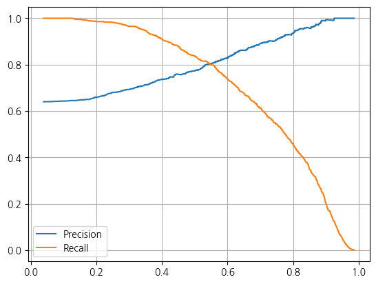
y_probaarray([[0.10658623, 0.89341377],
[0.22964498, 0.77035502],
[0.32770285, 0.67229715],
...,
[0.4013612 , 0.5986388 ],
[0.37399566, 0.62600434],
[0.57126278, 0.42873722]])2. Threshold 바꿔보기 (predict메서드의 기본 값은 0.5임)
from sklearn.preprocessing import Binarizer
binarizer = Binarizer(threshold = 0.525)
pred_bin = binarizer.transform(y_proba)[:,1]
pred_bin
array([1., 1., 1., ..., 1., 1., 0.])print(classification_report(y_test, pred_bin)) precision recall f1-score support
0 0.65 0.61 0.63 468
1 0.79 0.81 0.80 832
accuracy 0.74 1300
macro avg 0.72 0.71 0.72 1300
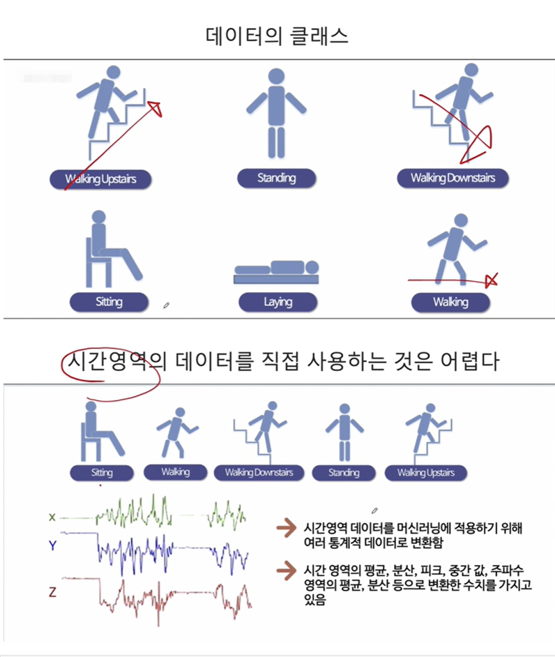
weighted avg 0.74 0.74 0.74 1300CH6-07 HAR 데이터 분석

feature_url = 'https://raw.githubusercontent.com/PinkWink/ML_tutorial/master/dataset/HAR_dataset/features.txt'
features = pd.read_csv(feature_url, sep = '\s+', header=None, index_col=False,names=['indexes','features'])
features| indexes | features | |
|---|---|---|
| 0 | 1 | tBodyAcc-mean()-X |
| 1 | 2 | tBodyAcc-mean()-Y |
| 2 | 3 | tBodyAcc-mean()-Z |
| 3 | 4 | tBodyAcc-std()-X |
| 4 | 5 | tBodyAcc-std()-Y |
| ... | ... | ... |
| 556 | 557 | angle(tBodyGyroMean,gravityMean) |
| 557 | 558 | angle(tBodyGyroJerkMean,gravityMean) |
| 558 | 559 | angle(X,gravityMean) |
| 559 | 560 | angle(Y,gravityMean) |
| 560 | 561 | angle(Z,gravityMean) |
561 rows × 2 columns
features.info()<class 'pandas.core.frame.DataFrame'>
RangeIndex: 561 entries, 0 to 560
Data columns (total 2 columns):
# Column Non-Null Count Dtype
--- ------ -------------- -----
0 indexes 561 non-null int64
1 features 561 non-null object
dtypes: int64(1), object(1)
memory usage: 8.9+ KBX_train_url = 'https://raw.githubusercontent.com/PinkWink/ML_tutorial/master/dataset/HAR_dataset/train/X_train.txt'
X_test_url = 'https://raw.githubusercontent.com/PinkWink/ML_tutorial/master/dataset/HAR_dataset/test/X_test.txt'
X_train = pd.read_csv(X_train_url, sep = '\s+',header=None)
X_test = pd.read_csv(X_test_url, sep = '\s+',header=None)X_train.info()
X_test.info()<class 'pandas.core.frame.DataFrame'>
RangeIndex: 7352 entries, 0 to 7351
Columns: 561 entries, 0 to 560
dtypes: float64(561)
memory usage: 31.5 MB
<class 'pandas.core.frame.DataFrame'>
RangeIndex: 2947 entries, 0 to 2946
Columns: 561 entries, 0 to 560
dtypes: float64(561)
memory usage: 12.6 MBX_train.columns = features.features.tolist()
X_test.columns = features.features.tolist()X_train.info()
X_test.info()<class 'pandas.core.frame.DataFrame'>
RangeIndex: 7352 entries, 0 to 7351
Columns: 561 entries, tBodyAcc-mean()-X to angle(Z,gravityMean)
dtypes: float64(561)
memory usage: 31.5 MB
<class 'pandas.core.frame.DataFrame'>
RangeIndex: 2947 entries, 0 to 2946
Columns: 561 entries, tBodyAcc-mean()-X to angle(Z,gravityMean)
dtypes: float64(561)
memory usage: 12.6 MBy_train_url = 'https://raw.githubusercontent.com/PinkWink/ML_tutorial/master/dataset/HAR_dataset/train/y_train.txt'
y_train = pd.read_csv(y_train_url, sep='\s+',header=None)
y_test_url = 'https://raw.githubusercontent.com/PinkWink/ML_tutorial/master/dataset/HAR_dataset/test/y_test.txt'
y_test = pd.read_csv(y_test_url, sep='\s+',header=None)
y_train.info()
y_test.info()<class 'pandas.core.frame.DataFrame'>
RangeIndex: 7352 entries, 0 to 7351
Data columns (total 1 columns):
# Column Non-Null Count Dtype
--- ------ -------------- -----
0 0 7352 non-null int64
dtypes: int64(1)
memory usage: 57.6 KB
<class 'pandas.core.frame.DataFrame'>
RangeIndex: 2947 entries, 0 to 2946
Data columns (total 1 columns):
# Column Non-Null Count Dtype
--- ------ -------------- -----
0 0 2947 non-null int64
dtypes: int64(1)
memory usage: 23.2 KBy_test.value_counts()6 537
5 532
1 496
4 491
2 471
3 420
Name: count, dtype: int64y_train.value_counts()6 1407
5 1374
4 1286
1 1226
2 1073
3 986
Name: count, dtype: int64y_train.columns = ['actions']
y_test.columns = ['actions']y_train.value_counts()actions
6 1407
5 1374
4 1286
1 1226
2 1073
3 986
Name: count, dtype: int64y_test.value_counts()actions
6    537
5    532
1    496
4    491
2    471
3    420
Name: count, dtype: int641.Train 데이터셋에 Decision Tree Grid Search 해보기
from sklearn.tree import DecisionTreeClassifier
dt = DecisionTreeClassifier(random_state=42)
from sklearn.model_selection import GridSearchCV
params = {'max_depth':[2,4,5,7,9,10,11,12,13,14,15]}
gs = GridSearchCV(dt,params,n_jobs=-1,cv=5,return_train_score=True)
gs.fit(X_train, y_train)
gs.best_score_0.8508001868320407gs.best_params_{'max_depth': 11}gs.cv_results_{'mean_fit_time': array([1.68399525, 3.15785847, 4.02245002, 5.50173416, 6.71298113,
7.33381157, 7.81237803, 8.29549851, 8.4962255 , 8.18297648,
7.2927084 ]),
'std_fit_time': array([0.01940284, 0.01585632, 0.07884301, 0.11550221, 0.21083578,
0.24150876, 0.16930031, 0.43835584, 0.3917013 , 0.53888856,
0.57083571]),
'mean_score_time': array([0.01250134, 0.01632829, 0.01076875, 0.0123621 , 0.01511126,
0.00774136, 0.01097193, 0.00937505, 0.00961781, 0.00613961,
0.00544543]),
'std_score_time': array([0.00625067, 0.00140205, 0.00947762, 0.00648656, 0.00266462,
0.0053481 , 0.01090915, 0.00765469, 0.00604583, 0.0067349 ,
0.00571478]),
'param_max_depth': masked_array(data=[2, 4, 5, 7, 9, 10, 11, 12, 13, 14, 15],
mask=[False, False, False, False, False, False, False, False,
False, False, False],
fill_value='?',
dtype=object),
'params': [{'max_depth': 2},
{'max_depth': 4},
{'max_depth': 5},
{'max_depth': 7},
{'max_depth': 9},
{'max_depth': 10},
{'max_depth': 11},
{'max_depth': 12},
{'max_depth': 13},
{'max_depth': 14},
{'max_depth': 15}],
'split0_test_score': array([0.54520734, 0.76206662, 0.80421482, 0.81305235, 0.81033311,
0.78653977, 0.80149558, 0.78925901, 0.79469748, 0.79537729,
0.79673691]),
'split1_test_score': array([0.54384772, 0.8735554 , 0.86471788, 0.83752549, 0.81849082,
0.80557444, 0.8171312 , 0.81849082, 0.81985044, 0.82732835,
0.82121006]),
'split2_test_score': array([0.54489796, 0.83673469, 0.83401361, 0.85170068, 0.84557823,
0.84013605, 0.85510204, 0.84489796, 0.84217687, 0.83877551,
0.84353741]),
'split3_test_score': array([0.54489796, 0.85170068, 0.85510204, 0.86666667, 0.87959184,
0.8829932 , 0.88911565, 0.87823129, 0.88707483, 0.89319728,
0.88435374]),
'split4_test_score': array([0.54421769, 0.87891156, 0.86734694, 0.87959184, 0.88639456,
0.88707483, 0.89115646, 0.88571429, 0.89931973, 0.8829932 ,
0.8829932 ]),
'mean_test_score': array([0.54461373, 0.84059379, 0.84507906, 0.8497074 , 0.84807771,
0.84046366, 0.85080019, 0.84331867, 0.84862387, 0.84753433,
0.84576627]),
'std_test_score': array([0.00050151, 0.04209392, 0.0235556 , 0.02313725, 0.03087914,
0.0402654 , 0.03655066, 0.03621503, 0.0395628 , 0.03618782,
0.03431236]),
'rank_test_score': array([11, 9, 7, 2, 4, 10, 1, 8, 3, 5, 6]),
'split0_train_score': array([0.54497534, 0.90647849, 0.92926373, 0.97857507, 0.98928754,
0.99234824, 0.99404863, 0.99557898, 0.99659922, 0.99710934,
0.99812957]),
'split1_train_score': array([0.54497534, 0.90103724, 0.91447033, 0.97160347, 0.99149804,
0.99591906, 0.99795953, 0.99863969, 0.99931984, 0.99948988,
0.99982996]),
'split2_train_score': array([0.54488269, 0.89221353, 0.92468548, 0.96718803, 0.99285957,
0.99455967, 0.99693982, 0.99761986, 0.99863992, 0.99914995,
0.99948997]),
'split3_train_score': array([0.5450527 , 0.89408365, 0.91193472, 0.96429786, 0.98860932,
0.99268956, 0.99557973, 0.99778987, 0.99863992, 0.99914995,
0.99948997]),
'split4_train_score': array([0.54522271, 0.90343421, 0.92196532, 0.96157769, 0.98690921,
0.99149949, 0.99387963, 0.99625978, 0.99812989, 0.99897994,
0.99948997]),
'mean_train_score': array([0.54502176, 0.89944942, 0.92046391, 0.96864842, 0.98983274,
0.99340321, 0.99568147, 0.99717763, 0.99826576, 0.99877581,
0.99928589]),
'std_train_score': array([0.00011401, 0.00545815, 0.00642157, 0.00597204, 0.00211073,
0.00160707, 0.00159349, 0.00110509, 0.00091509, 0.00084955,
0.00059296])}val_scores = gs.cv_results_['mean_test_score']
val_train_scores = gs.cv_results_['mean_train_score']
val_scores_df = pd.DataFrame({'max_depth':params['max_depth'],
'mean_val_scores':val_scores,
'mean_train_scores':val_train_scores})val_scores_df| max_depth | mean_val_scores | mean_train_scores | |
|---|---|---|---|
| 0 | 2 | 0.544614 | 0.545022 |
| 1 | 4 | 0.840594 | 0.899449 |
| 2 | 5 | 0.845079 | 0.920464 |
| 3 | 7 | 0.849707 | 0.968648 |
| 4 | 9 | 0.848078 | 0.989833 |
| 5 | 10 | 0.840464 | 0.993403 |
| 6 | 11 | 0.850800 | 0.995681 |
| 7 | 12 | 0.843319 | 0.997178 |
| 8 | 13 | 0.848624 | 0.998266 |
| 9 | 14 | 0.847534 | 0.998776 |
| 10 | 15 | 0.845766 | 0.999286 |
2. Test 데이터셋에 해보기
params = {'max_depth':[2,4,6,8,9,10,11,12,13,14]}for i in params['max_depth']:
dt = DecisionTreeClassifier(max_depth=i, random_state=42)
dt.fit(X_train,y_train)
pred = dt.predict(X_test)
accuracy = accuracy_score(y_test,pred)
print('max_depth: ', i, 'Accuracy_score: ',accuracy)max_depth: 2 Accuracy_score: 0.5310485239226331
max_depth: 4 Accuracy_score: 0.8096369189005769
max_depth: 6 Accuracy_score: 0.8544282321004412
max_depth: 8 Accuracy_score: 0.8683406854428232
max_depth: 9 Accuracy_score: 0.8700373260943333
max_depth: 10 Accuracy_score: 0.8625721072276892
max_depth: 11 Accuracy_score: 0.8686800135731252
max_depth: 12 Accuracy_score: 0.8642687478791992
max_depth: 13 Accuracy_score: 0.8605361384458772
max_depth: 14 Accuracy_score: 0.8527315914489311y_test_array = np.array(y_test).reshape(-1)
y_train_array = np.array(y_train).reshape(-1)3. 랜덤포레스트에 적용시켜보기
from sklearn.ensemble import RandomForestClassifier
rf = RandomForestClassifier(random_state=42)
params = {'max_depth':[2,4,6,8,10,12,14,16],
          'n_estimators':[90,120,150],
          'min_samples_split':[4,8],
          'min_samples_leaf':[4,8]}
gs = GridSearchCV(rf, params, n_jobs=-1,verbose=2)
gs.fit(X_train,y_train_array)
y_pred = gs.predict(X_test)
accuracy = accuracy_score(y_test_array,y_pred)Fitting 5 folds for each of 96 candidates, totalling 480 fitsaccuracy0.9236511706820495gs.best_params_{'max_depth': 14,
'min_samples_leaf': 8,
'min_samples_split': 4,
'n_estimators': 150}best_score = gs.cv_results_['mean_test_score'].mean()best_score0.9006998879316059best_model = gs.best_estimator_feature_importances = best_model.feature_importances_.tolist()
features = X_train.columns.tolist()feature_importances = pd.DataFrame({'features':features,
'feature_importances':feature_importances})feature_importances.sort_values(by = 'feature_importances', ascending=False).head(20)| features | feature_importances | |
|---|---|---|
| 40 | tGravityAcc-mean()-X | 0.035414 |
| 558 | angle(X,gravityMean) | 0.033220 |
| 52 | tGravityAcc-min()-X | 0.031955 |
| 56 | tGravityAcc-energy()-X | 0.029643 |
| 41 | tGravityAcc-mean()-Y | 0.027789 |
| 49 | tGravityAcc-max()-X | 0.026918 |
| 53 | tGravityAcc-min()-Y | 0.025761 |
| 50 | tGravityAcc-max()-Y | 0.022822 |
| 559 | angle(Y,gravityMean) | 0.020196 |
| 57 | tGravityAcc-energy()-Y | 0.015482 |
| 560 | angle(Z,gravityMean) | 0.012863 |
| 83 | tBodyAccJerk-std()-X | 0.012111 |
| 353 | fBodyAccJerk-max()-X | 0.012101 |
| 360 | fBodyAccJerk-energy()-X | 0.011890 |
| 271 | fBodyAcc-mad()-X | 0.011734 |
| 389 | fBodyAccJerk-bandsEnergy()-1,16 | 0.010640 |
| 503 | fBodyAccMag-std() | 0.009779 |
| 504 | fBodyAccMag-mad() | 0.009763 |
| 54 | tGravityAcc-min()-Z | 0.009480 |
| 181 | tBodyGyroJerk-iqr()-Z | 0.008942 |
feature_importances.set_index('features',inplace=True)feature_importances.sort_values(by = 'feature_importances', ascending=False).head(20).plot(kind='barh',colormap='RdBu')<Axes: ylabel='features'>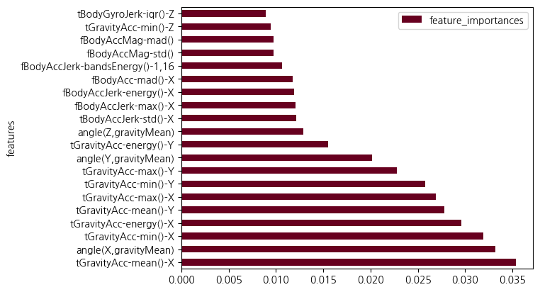
best_features = np.array(feature_importances.sort_values(by='feature_importances', ascending=False).head(20).index)4. 피처 중요도가 상위 20개인 것만 가지고 GridSearchCV로 찾은 bestmodel로 예측하기
best_featuresarray(['tGravityAcc-mean()-X', 'angle(X,gravityMean)',
'tGravityAcc-min()-X', 'tGravityAcc-energy()-X',
'tGravityAcc-mean()-Y', 'tGravityAcc-max()-X',
'tGravityAcc-min()-Y', 'tGravityAcc-max()-Y',
'angle(Y,gravityMean)', 'tGravityAcc-energy()-Y',
'angle(Z,gravityMean)', 'tBodyAccJerk-std()-X',
'fBodyAccJerk-max()-X', 'fBodyAccJerk-energy()-X',
'fBodyAcc-mad()-X', 'fBodyAccJerk-bandsEnergy()-1,16',
'fBodyAccMag-std()', 'fBodyAccMag-mad()', 'tGravityAcc-min()-Z',
'tBodyGyroJerk-iqr()-Z'], dtype=object)X_train_re = X_train[best_features]
X_test_re = X_test[best_features]best_model.fit(X_train_re,np.array(y_train).reshape(-1))
y_pred_re = best_model.predict(X_test_re)5. 피처 중요도 상위 20개만 추려서 아까 추출한 bestestimator에 적합시키면 Accuracy는 0.81정도로 0.1정도 떨어지는 모습임
print('Accuracy Score: ', accuracy_score(y_test, y_pred_re))Accuracy Score: 0.8103155751611809CH7-01 wine데이터로 부스팅 모델 적용 및 예측하기 타겟칼럼을 taste로
from sklearn.metrics import roc_auc_score, roc_curve, RocCurveDisplay, f1_score, accuracy_score, recall_score, precision_score
from sklearn.ensemble import RandomForestClassifier
import pandas as pd
import numpy as np

url_w = 'https://archive.ics.uci.edu/ml/machine-learning-databases/wine-quality/winequality-white.csv'
url_r = 'https://archive.ics.uci.edu/ml/machine-learning-databases/wine-quality/winequality-red.csv'
white_df = pd.read_csv(url_w,sep=';')
red_df = pd.read_csv(url_r,sep=';')
wine_df = pd.concat([white_df, red_df], axis = 0)
wine_df['taste'] = wine_df['quality'].apply(lambda x: 1 if x>5 else 0)
wine_df.info()<class 'pandas.core.frame.DataFrame'>
Index: 6497 entries, 0 to 1598
Data columns (total 13 columns):
# Column Non-Null Count Dtype
--- ------ -------------- -----
0 fixed acidity 6497 non-null float64
1 volatile acidity 6497 non-null float64
2 citric acid 6497 non-null float64
3 residual sugar 6497 non-null float64
4 chlorides 6497 non-null float64
5 free sulfur dioxide 6497 non-null float64
6 total sulfur dioxide 6497 non-null float64
7 density 6497 non-null float64
8 pH 6497 non-null float64
9 sulphates 6497 non-null float64
10 alcohol 6497 non-null float64
11 quality 6497 non-null int64
12 taste 6497 non-null int64
dtypes: float64(11), int64(2)
memory usage: 710.6 KB1. StandardScaler 로 표준화하기
X = wine_df.drop(['quality','taste'],axis=1)
y = wine_df['taste']
from sklearn.preprocessing import StandardScaler
ss = StandardScaler()
X_sc = ss.fit_transform(X)from sklearn.model_selection import train_test_split
X_train, X_test, y_train, y_test = train_test_split(X_sc,y,test_size=0.2, stratify=y, random_state=2024)wine_df.hist(bins=10, figsize=(15,10))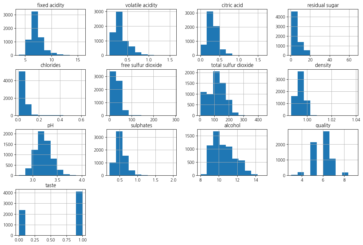
2. quality별 특성과의 상관관계를 보자
corr_matrix = wine_df.corr(method='pearson')pd.pivot_table(wine_df,index='quality',values=X.columns,aggfunc='median')| alcohol | chlorides | citric acid | density | fixed acidity | free sulfur dioxide | pH | residual sugar | sulphates | total sulfur dioxide | volatile acidity | |
|---|---|---|---|---|---|---|---|---|---|---|---|
| quality | |||||||||||
| 3 | 10.15 | 0.0550 | 0.33 | 0.995900 | 7.45 | 17.0 | 3.245 | 3.15 | 0.505 | 102.5 | 0.415 |
| 4 | 10.00 | 0.0505 | 0.26 | 0.994995 | 7.00 | 15.0 | 3.220 | 2.20 | 0.485 | 102.0 | 0.380 |
| 5 | 9.60 | 0.0530 | 0.30 | 0.996100 | 7.10 | 27.0 | 3.190 | 3.00 | 0.500 | 127.0 | 0.330 |
| 6 | 10.50 | 0.0460 | 0.31 | 0.994700 | 6.90 | 29.0 | 3.210 | 3.10 | 0.510 | 117.0 | 0.270 |
| 7 | 11.40 | 0.0390 | 0.32 | 0.992400 | 6.90 | 30.0 | 3.220 | 2.80 | 0.520 | 114.0 | 0.270 |
| 8 | 12.00 | 0.0370 | 0.32 | 0.991890 | 6.80 | 34.0 | 3.230 | 4.10 | 0.480 | 118.0 | 0.280 |
| 9 | 12.50 | 0.0310 | 0.36 | 0.990300 | 7.10 | 28.0 | 3.280 | 2.20 | 0.460 | 119.0 | 0.270 |
corr_matrix['quality'].sort_values(ascending=False)quality 1.000000
taste 0.814484
alcohol 0.444319
citric acid 0.085532
free sulfur dioxide 0.055463
sulphates 0.038485
pH 0.019506
residual sugar -0.036980
total sulfur dioxide -0.041385
fixed acidity -0.076743
chlorides -0.200666
volatile acidity -0.265699
density -0.305858
Name: quality, dtype: float643. taste의 분포
sns.countplot(data=wine_df, x='taste',hue='taste')<Axes: xlabel='taste', ylabel='count'>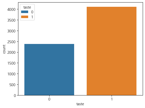
4. 다양한 모델들을 한 번에 테스트하기
from sklearn.model_selection import KFold
from sklearn.ensemble import GradientBoostingClassifier, AdaBoostClassifier, RandomForestClassifier
from sklearn.linear_model import LogisticRegression
from sklearn.tree import DecisionTreeClassifier
models = []
models.append(('GradientBoostingClassifier', GradientBoostingClassifier()))
models.append(('AdaBoostClassifier', AdaBoostClassifier()))
models.append(('RandomForestClassifier', RandomForestClassifier()))
models.append(('LogisticRegression', LogisticRegression()))
models.append(('DecisionTreeClassifier', DecisionTreeClassifier()))from sklearn.model_selection import cross_val_scoreresults = []
names = []
for name, model in models:
kfold = KFold(n_splits=5, shuffle=True, random_state=2024)
cv_results = cross_val_score(model,X_train,y_train,scoring='accuracy',cv=kfold,n_jobs=-1, verbose=2)
results.append(cv_results)
names.append(name)
print(name, cv_results.mean(), cv_results.std())[Parallel(n_jobs=-1)]: Using backend LokyBackend with 16 concurrent workers.
[Parallel(n_jobs=-1)]: Done 5 out of 5 | elapsed: 2.3s finished
[Parallel(n_jobs=-1)]: Using backend LokyBackend with 16 concurrent workers.
GradientBoostingClassifier 0.7696759087880358 0.008838681565602958
[Parallel(n_jobs=-1)]: Done 5 out of 5 | elapsed: 1.1s finished
[Parallel(n_jobs=-1)]: Using backend LokyBackend with 16 concurrent workers.
AdaBoostClassifier 0.7554364403642555 0.010739534578889818
[Parallel(n_jobs=-1)]: Done 5 out of 5 | elapsed: 2.0s finished
[Parallel(n_jobs=-1)]: Using backend LokyBackend with 16 concurrent workers.
RandomForestClassifier 0.8237437995113644 0.0076948907495272304
LogisticRegression 0.7385042940697415 0.015459699390032468
DecisionTreeClassifier 0.7648672910342784 0.01670975301458157
[Parallel(n_jobs=-1)]: Done 5 out of 5 | elapsed: 0.7s finished
[Parallel(n_jobs=-1)]: Using backend LokyBackend with 16 concurrent workers.
[Parallel(n_jobs=-1)]: Done 5 out of 5 | elapsed: 0.0s finishedresults[array([0.77980769, 0.75384615, 0.77574591, 0.76997113, 0.76900866]),
array([0.76538462, 0.74230769, 0.76708373, 0.74302214, 0.75938402]),
array([0.83557692, 0.81538462, 0.8267565 , 0.82579403, 0.81520693]),
array([0.75 , 0.72019231, 0.74302214, 0.72088547, 0.75842156]),
array([0.78076923, 0.73365385, 0.76708373, 0.77767084, 0.76515881])]names['GradientBoostingClassifier',
'AdaBoostClassifier',
'RandomForestClassifier',
'LogisticRegression',
'DecisionTreeClassifier']fig = plt.figure(figsize=(10,10))
plt.suptitle('Algorithm Comparison')
ax = fig.add_subplot(111)
plt.boxplot(results)
ax.set_xticklabels(labels=names)
plt.show()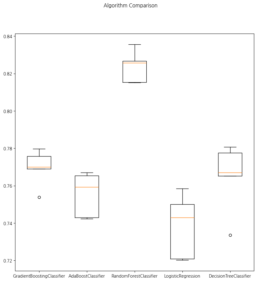
5. 테스트 데이터에 대한 결과 평가
for name, model in models:
    model.fit(X_train,y_train)
    pred = model.predict(X_test)

    print(name, accuracy_score(y_test, pred))
GradientBoostingClassifier 0.7715384615384615
AdaBoostClassifier 0.7561538461538462
RandomForestClassifier 0.8323076923076923
LogisticRegression 0.73
DecisionTreeClassifier 0.7753846153846153CH7-01 KNN(K-Nearest Neighbor)
1. 거리기반 알고리즘이기 때문에 단위의 스케일링이 학습에 엄청난 영향을 미치므로 반드시 피처간 스케일링을 해줘야 함