from sklearn.datasets import load_iris
import pandas as pd
import numpy as np
import sklearn
import matplotlib.pyplot as plt
import koreanize_matplotlib
import seaborn as sns
CH1-02~CH1-03: sklearn의 Iris데이터셋 불러오고 살펴보기
1-1. sklearn의 iris데이터셋 불러오기
iris_raw = sklearn.datasets.load_iris()print(iris_raw['DESCR']).. _iris_dataset:
Iris plants dataset
--------------------
**Data Set Characteristics:**
:Number of Instances: 150 (50 in each of three classes)
:Number of Attributes: 4 numeric, predictive attributes and the class
:Attribute Information:
- sepal length in cm
- sepal width in cm
- petal length in cm
- petal width in cm
- class:
- Iris-Setosa
- Iris-Versicolour
- Iris-Virginica
:Summary Statistics:
============== ==== ==== ======= ===== ====================
Min Max Mean SD Class Correlation
============== ==== ==== ======= ===== ====================
sepal length: 4.3 7.9 5.84 0.83 0.7826
sepal width: 2.0 4.4 3.05 0.43 -0.4194
petal length: 1.0 6.9 3.76 1.76 0.9490 (high!)
petal width: 0.1 2.5 1.20 0.76 0.9565 (high!)
============== ==== ==== ======= ===== ====================
:Missing Attribute Values: None
:Class Distribution: 33.3% for each of 3 classes.
:Creator: R.A. Fisher
:Donor: Michael Marshall (MARSHALL%PLU@io.arc.nasa.gov)
:Date: July, 1988
The famous Iris database, first used by Sir R.A. Fisher. The dataset is taken
from Fisher's paper. Note that it's the same as in R, but not as in the UCI
Machine Learning Repository, which has two wrong data points.
This is perhaps the best known database to be found in the
pattern recognition literature. Fisher's paper is a classic in the field and
is referenced frequently to this day. (See Duda & Hart, for example.) The
data set contains 3 classes of 50 instances each, where each class refers to a
type of iris plant. One class is linearly separable from the other 2; the
latter are NOT linearly separable from each other.
|details-start|
**References**
|details-split|
- Fisher, R.A. "The use of multiple measurements in taxonomic problems"
Annual Eugenics, 7, Part II, 179-188 (1936); also in "Contributions to
Mathematical Statistics" (John Wiley, NY, 1950).
- Duda, R.O., & Hart, P.E. (1973) Pattern Classification and Scene Analysis.
(Q327.D83) John Wiley & Sons. ISBN 0-471-22361-1. See page 218.
- Dasarathy, B.V. (1980) "Nosing Around the Neighborhood: A New System
Structure and Classification Rule for Recognition in Partially Exposed
Environments". IEEE Transactions on Pattern Analysis and Machine
Intelligence, Vol. PAMI-2, No. 1, 67-71.
- Gates, G.W. (1972) "The Reduced Nearest Neighbor Rule". IEEE Transactions
on Information Theory, May 1972, 431-433.
- See also: 1988 MLC Proceedings, 54-64. Cheeseman et al"s AUTOCLASS II
conceptual clustering system finds 3 classes in the data.
- Many, many more ...
|details-end|1-2. iris의 타겟과 피처를 데이터프레임으로 저장하기
X, y = iris_raw['data'], iris_raw['target']iris_df = pd.DataFrame(X, columns = iris_raw['feature_names'])
iris_df.head()| sepal length (cm) | sepal width (cm) | petal length (cm) | petal width (cm) | |
|---|---|---|---|---|
| 0 | 5.1 | 3.5 | 1.4 | 0.2 |
| 1 | 4.9 | 3.0 | 1.4 | 0.2 |
| 2 | 4.7 | 3.2 | 1.3 | 0.2 |
| 3 | 4.6 | 3.1 | 1.5 | 0.2 |
| 4 | 5.0 | 3.6 | 1.4 | 0.2 |
iris_df['species'] = iris_raw['target']
iris_df.info()<class 'pandas.core.frame.DataFrame'>
RangeIndex: 150 entries, 0 to 149
Data columns (total 5 columns):
# Column Non-Null Count Dtype
--- ------ -------------- -----
0 sepal length (cm) 150 non-null float64
1 sepal width (cm) 150 non-null float64
2 petal length (cm) 150 non-null float64
3 petal width (cm) 150 non-null float64
4 species 150 non-null int32
dtypes: float64(4), int32(1)
memory usage: 5.4 KBiris_df| sepal length (cm) | sepal width (cm) | petal length (cm) | petal width (cm) | species | |
|---|---|---|---|---|---|
| 0 | 5.1 | 3.5 | 1.4 | 0.2 | 0 |
| 1 | 4.9 | 3.0 | 1.4 | 0.2 | 0 |
| 2 | 4.7 | 3.2 | 1.3 | 0.2 | 0 |
| 3 | 4.6 | 3.1 | 1.5 | 0.2 | 0 |
| 4 | 5.0 | 3.6 | 1.4 | 0.2 | 0 |
| ... | ... | ... | ... | ... | ... |
| 145 | 6.7 | 3.0 | 5.2 | 2.3 | 2 |
| 146 | 6.3 | 2.5 | 5.0 | 1.9 | 2 |
| 147 | 6.5 | 3.0 | 5.2 | 2.0 | 2 |
| 148 | 6.2 | 3.4 | 5.4 | 2.3 | 2 |
| 149 | 5.9 | 3.0 | 5.1 | 1.8 | 2 |
150 rows × 5 columns
iris_df.describe()| sepal length (cm) | sepal width (cm) | petal length (cm) | petal width (cm) | species | |
|---|---|---|---|---|---|
| count | 150.000000 | 150.000000 | 150.000000 | 150.000000 | 150.000000 |
| mean | 5.843333 | 3.057333 | 3.758000 | 1.199333 | 1.000000 |
| std | 0.828066 | 0.435866 | 1.765298 | 0.762238 | 0.819232 |
| min | 4.300000 | 2.000000 | 1.000000 | 0.100000 | 0.000000 |
| 25% | 5.100000 | 2.800000 | 1.600000 | 0.300000 | 0.000000 |
| 50% | 5.800000 | 3.000000 | 4.350000 | 1.300000 | 1.000000 |
| 75% | 6.400000 | 3.300000 | 5.100000 | 1.800000 | 2.000000 |
| max | 7.900000 | 4.400000 | 6.900000 | 2.500000 | 2.000000 |
1-3. boxplot(sepal length와 species와의 관계)
sns.boxplot(data = iris_df, y = 'sepal length (cm)', x = 'species')<Axes: xlabel='species', ylabel='sepal length (cm)'>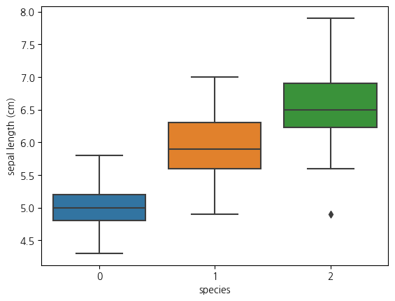
1-4. boxplot(sepal width와 species와의 관계)
sns.boxplot(data = iris_df, x = 'species', y = 'sepal width (cm)') <Axes: xlabel='species', ylabel='sepal width (cm)'>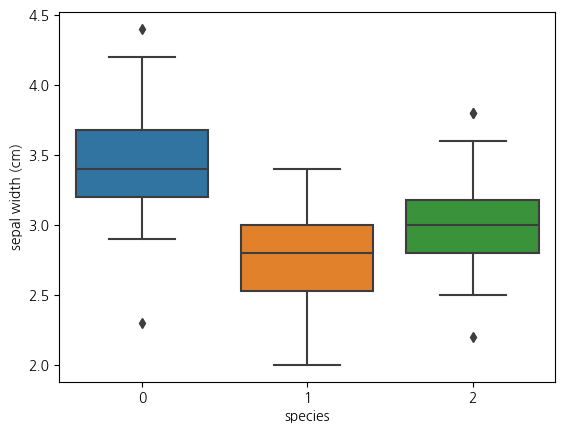
1-5. boxplot(petal length와 species와의 관계)
sns.boxplot(data=iris_df, y='petal length (cm)', x='species')<Axes: xlabel='species', ylabel='petal length (cm)'>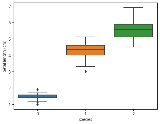
1-6. boxplot(petal width와 species와의 관계)
sns.boxplot(data=iris_df, x='species', y='petal width (cm)')<Axes: xlabel='species', ylabel='petal width (cm)'>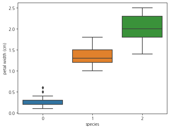
1-6. pairplot 그려보기
sns.pairplot(iris_df, hue = 'species', palette= 'Set1')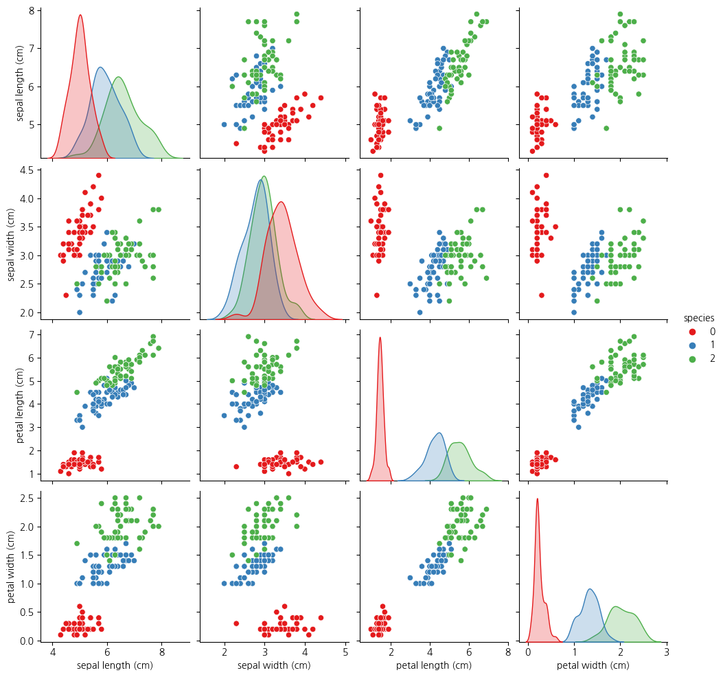
1-7. pairplot에서 petal width와 petal length의 산점도를 보면 3개 종 구분이 가능해보임
sns.lmplot(iris_df, x='petal length (cm)', y='petal width (cm)', hue='species')<seaborn.axisgrid.FacetGrid at 0x15bf62caf10>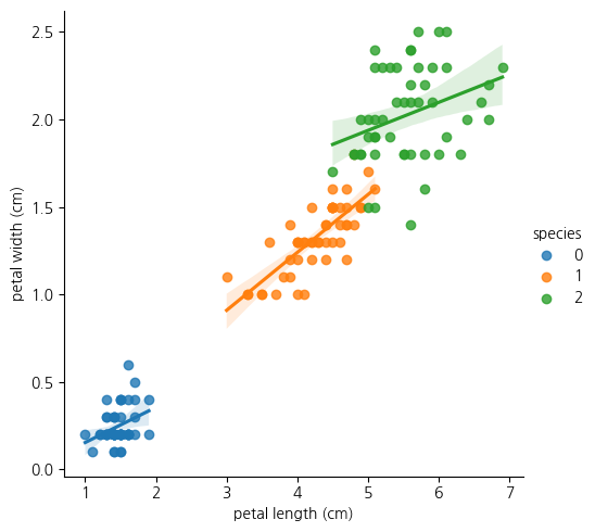
1-8.위의 lmplot을 분석해보면 species가 0인 클래스는 petal length가 다 2이하임
- 또한 클래스 1의 경우 petal length가 대체로 3~5사이에 있음
- 클래스 2의 경우 petal width가 1.6정도 이상에 거의 분포
Decision Tree로 그려보자
CH1-04: Decision Tree를 살펴보자
2-01: Scatterplot(petal length와 petal width사이의 관계보기)
plt.figure(figsize=(12,6))
sns.scatterplot(iris_df, x='petal length (cm)', y='petal width (cm)', hue = 'species', palette = 'Set1')
plt.show()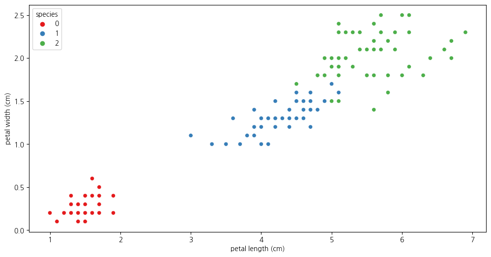
2-2. species가 0인 것을 제외하고 살펴보기
iris_12 = iris_df.loc[iris_df['species']!=0]
iris_12.info()<class 'pandas.core.frame.DataFrame'>
Index: 100 entries, 50 to 149
Data columns (total 5 columns):
# Column Non-Null Count Dtype
--- ------ -------------- -----
0 sepal length (cm) 100 non-null float64
1 sepal width (cm) 100 non-null float64
2 petal length (cm) 100 non-null float64
3 petal width (cm) 100 non-null float64
4 species 100 non-null int32
dtypes: float64(4), int32(1)
memory usage: 4.3 KBiris_12| sepal length (cm) | sepal width (cm) | petal length (cm) | petal width (cm) | species | |
|---|---|---|---|---|---|
| 50 | 7.0 | 3.2 | 4.7 | 1.4 | 1 |
| 51 | 6.4 | 3.2 | 4.5 | 1.5 | 1 |
| 52 | 6.9 | 3.1 | 4.9 | 1.5 | 1 |
| 53 | 5.5 | 2.3 | 4.0 | 1.3 | 1 |
| 54 | 6.5 | 2.8 | 4.6 | 1.5 | 1 |
| ... | ... | ... | ... | ... | ... |
| 145 | 6.7 | 3.0 | 5.2 | 2.3 | 2 |
| 146 | 6.3 | 2.5 | 5.0 | 1.9 | 2 |
| 147 | 6.5 | 3.0 | 5.2 | 2.0 | 2 |
| 148 | 6.2 | 3.4 | 5.4 | 2.3 | 2 |
| 149 | 5.9 | 3.0 | 5.1 | 1.8 | 2 |
100 rows × 5 columns
2-3. species가 1,2 인 것에 대해 scatterplot 살펴보기
- 두 품종을 어느 기준으로 분할할지 생각해보기
plt.figure(figsize=(12,6))
sns.scatterplot(data=iris_12, x='petal length (cm)', y='petal width (cm)', hue = 'species')<Axes: xlabel='petal length (cm)', ylabel='petal width (cm)'>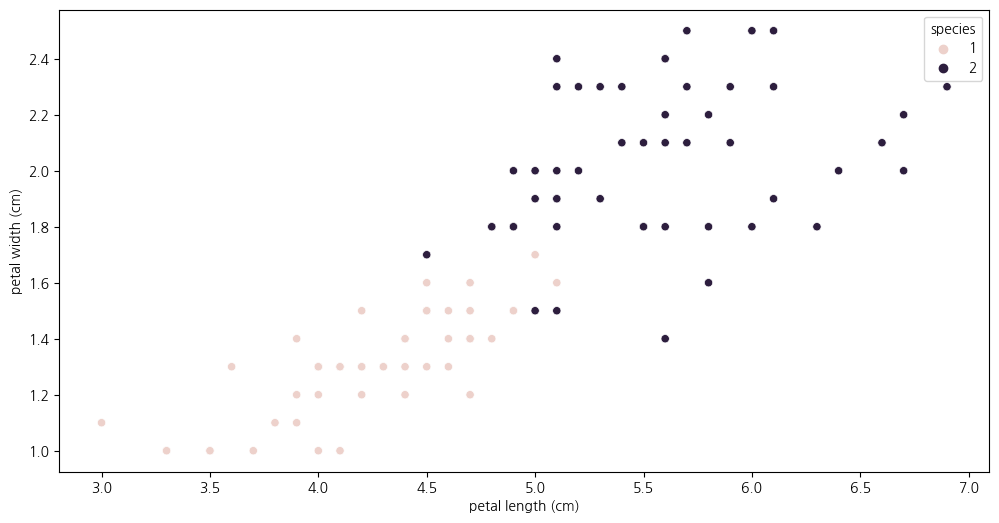
2-4. Decision Tree의 분할 기준(split criteria)
주로 엔트로피 또는 지니불순도로 분할함
- 정보이득(information gain)
- 엔트로피 불순도를 기준으로 impurity가 작은 방향으로 계속 가지를 뻗어나감
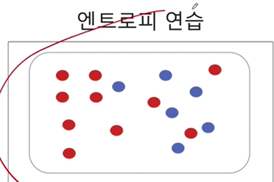
2-5. 엔트로피란?

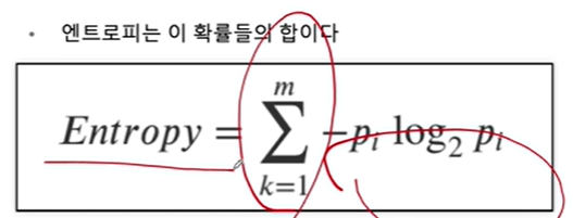
- 여기서 p는 해당 데이터포인트가 해당 클래스에 속할 확률
- 어떤 확률 분포로 일어나는 사건을 표현할 때 필요한 정보의 양
- 이 값이 커질수록 결과에 대한 예측이 어려워짐
2-6. 엔트로피 계산 연습

-(10/16) * np.log2(10/16) - (6/16) * np.log2(6/16)0.954434002924965만약에 디시젼트리처럼 노드 하나를 두 부분으로 분할하면
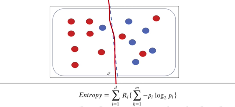
# 왼쪽 부분의 엔트로피(0.5를 곱해주는 것은 두 부분 중 하나를 선택할 확률)
0.5 * (-(7/8)*np.log2(7/8) - (1/8)*np.log2(1/8)) +\
0.5 * (-(3/8)*np.log2(3/8) - (5/8)*np.log2(5/8))0.7489992230622807두 덩어리로 분리한 엔트로피가 한 덩어리였던 엔트로피보다 내려갔으므로
- 엔트로피가 내려간다는 것은 정보불순도가 감소한다는 것으로 타겟을 맞출 확률이 높아진다는 것
- 두 덩어리로 나누는 게 더 좋다
2-7. 지니불순도를 계산해보자
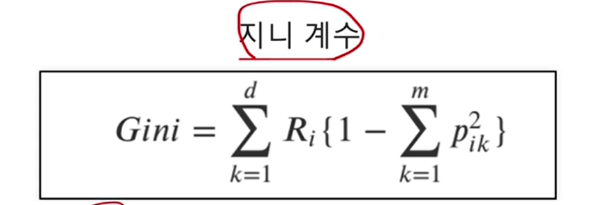
1-((10/16)**2 + (6/16) ** 2)0.46875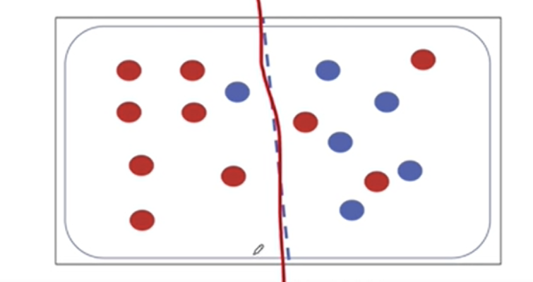
(0.5)*(1-((1/8)**2 + (7/8)**2) + (1-((3/8)**2 + (5/8)**2)))0.34375지니불순도의 경우에도 불순도가 감소하였으므로 두 덩어리로 나누는게 더 낫다
[참고] 정보이득(Information Gain)이란?
정보이득이란: {부모노드- (자식노드불순도(지니 or 엔트로피)의 가중평균)}

CH1-07(1): Decision Tree 학습 해보기(일단은 petal length, petal width 피처만 사용하여)
from sklearn.tree import DecisionTreeClassifierdt = DecisionTreeClassifier(max_depth = 2, criterion ='entropy', random_state=2024)7-1.Train셋과 Test셋으로 분리해보기(보통 8:2의 비율을 많이 씀)
- 클래스 불균형을 막기위해 train_test_split의 stratify 파라미터에 타겟값(train, test의 합친세트)를 넣어주기
from sklearn.model_selection import train_test_splitX_train, X_test, y_train, y_test = train_test_split(X[:,2:], y,
stratify = y, test_size=0.2, random_state=2024)7-2.DecisionTree를 학습하고 테스트 셋과 트레인셋의 Accuracy Score 보기
# 테스트셋의 Accuracy Score
dt.fit(X_train, y_train)
dt.score(X_test, y_test)0.9333333333333333y_train_pred = dt.predict(X_train)7-3. trainset의 타겟을 예측한 Accuracy Score 0.9583이고
- testset을 예측한 Accuracy Score가 0.9333이므로 과적합은 아님
from sklearn.metrics import accuracy_score
accuracy_score(y_train, y_train_pred)0.95833333333333347-4. X_test을 통해 예측된 y(타겟)값들 보기
y_pred = dt.predict(X_test)
y_pred
array([0, 2, 0, 1, 2, 0, 2, 1, 0, 1, 0, 1, 2, 2, 2, 2, 2, 0, 0, 1, 1, 1,
1, 0, 1, 2, 0, 0, 2, 1])7-5.DecisionTree개체에 내장된 속성인 predict_proba를 통해
- X_train의 각 데이터(샘플, 행)들에서 3개의 species를 선택할 확률을 보자
dt.predict_proba(X_train)array([[1. , 0. , 0. ],
[0. , 1. , 0. ],
[0. , 0.11111111, 0.88888889],
[1. , 0. , 0. ],
[1. , 0. , 0. ],
[0. , 1. , 0. ],
[0. , 1. , 0. ],
[0. , 0.11111111, 0.88888889],
[1. , 0. , 0. ],
[0. , 1. , 0. ],
[1. , 0. , 0. ],
[0. , 0.11111111, 0.88888889],
[0. , 1. , 0. ],
[0. , 0.11111111, 0.88888889],
[0. , 0.11111111, 0.88888889],
[0. , 0.11111111, 0.88888889],
[0. , 1. , 0. ],
[0. , 0.11111111, 0.88888889],
[1. , 0. , 0. ],
[0. , 0.11111111, 0.88888889],
[1. , 0. , 0. ],
[1. , 0. , 0. ],
[0. , 0.11111111, 0.88888889],
[0. , 0.11111111, 0.88888889],
[0. , 1. , 0. ],
[0. , 0.11111111, 0.88888889],
[0. , 1. , 0. ],
[0. , 1. , 0. ],
[0. , 1. , 0. ],
[1. , 0. , 0. ],
[1. , 0. , 0. ],
[0. , 0.11111111, 0.88888889],
[0. , 0.11111111, 0.88888889],
[0. , 1. , 0. ],
[0. , 0.11111111, 0.88888889],
[1. , 0. , 0. ],
[0. , 1. , 0. ],
[0. , 1. , 0. ],
[0. , 0.11111111, 0.88888889],
[0. , 0.11111111, 0.88888889],
[0. , 0.11111111, 0.88888889],
[1. , 0. , 0. ],
[0. , 0.11111111, 0.88888889],
[0. , 1. , 0. ],
[1. , 0. , 0. ],
[0. , 1. , 0. ],
[0. , 1. , 0. ],
[1. , 0. , 0. ],
[0. , 1. , 0. ],
[0. , 0.11111111, 0.88888889],
[0. , 1. , 0. ],
[0. , 1. , 0. ],
[1. , 0. , 0. ],
[0. , 1. , 0. ],
[0. , 0.11111111, 0.88888889],
[0. , 0.11111111, 0.88888889],
[1. , 0. , 0. ],
[0. , 0.11111111, 0.88888889],
[1. , 0. , 0. ],
[0. , 0.11111111, 0.88888889],
[1. , 0. , 0. ],
[1. , 0. , 0. ],
[0. , 1. , 0. ],
[0. , 1. , 0. ],
[1. , 0. , 0. ],
[0. , 0.11111111, 0.88888889],
[0. , 0.11111111, 0.88888889],
[1. , 0. , 0. ],
[0. , 0.11111111, 0.88888889],
[1. , 0. , 0. ],
[0. , 1. , 0. ],
[0. , 1. , 0. ],
[0. , 1. , 0. ],
[0. , 1. , 0. ],
[0. , 1. , 0. ],
[1. , 0. , 0. ],
[0. , 0.11111111, 0.88888889],
[0. , 0.11111111, 0.88888889],
[0. , 0.11111111, 0.88888889],
[0. , 0.11111111, 0.88888889],
[0. , 0.11111111, 0.88888889],
[0. , 0.11111111, 0.88888889],
[1. , 0. , 0. ],
[1. , 0. , 0. ],
[1. , 0. , 0. ],
[0. , 0.11111111, 0.88888889],
[0. , 0.11111111, 0.88888889],
[0. , 0.11111111, 0.88888889],
[1. , 0. , 0. ],
[0. , 0.11111111, 0.88888889],
[0. , 0.11111111, 0.88888889],
[0. , 1. , 0. ],
[0. , 0.11111111, 0.88888889],
[0. , 0.11111111, 0.88888889],
[0. , 0.11111111, 0.88888889],
[0. , 0.11111111, 0.88888889],
[1. , 0. , 0. ],
[0. , 1. , 0. ],
[0. , 0.11111111, 0.88888889],
[0. , 1. , 0. ],
[0. , 0.11111111, 0.88888889],
[1. , 0. , 0. ],
[0. , 0.11111111, 0.88888889],
[1. , 0. , 0. ],
[1. , 0. , 0. ],
[0. , 1. , 0. ],
[0. , 1. , 0. ],
[1. , 0. , 0. ],
[1. , 0. , 0. ],
[1. , 0. , 0. ],
[0. , 1. , 0. ],
[0. , 0.11111111, 0.88888889],
[1. , 0. , 0. ],
[1. , 0. , 0. ],
[0. , 1. , 0. ],
[1. , 0. , 0. ],
[1. , 0. , 0. ],
[1. , 0. , 0. ],
[0. , 1. , 0. ],
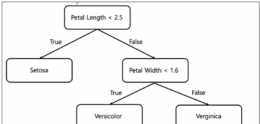
[1. , 0. , 0. ]])7-6. DecisionTree모델이 어떻게 가지를 뻗어나갔는지 시각화해보자
from sklearn.tree import plot_treeplt.figure(figsize=(15,15))
plot_tree(dt,label='all',feature_names=iris_raw['feature_names'][2:],\
filled=True, precision=3);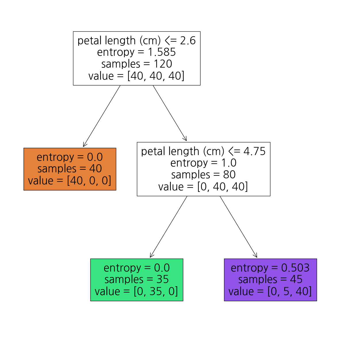
7-7. mlxtend를 활용하여 산점도와 함께 DecisionTree가 나뉜 기준 시각화해보기
7-8. trainset에 대한 DecisionTree의 결정경계 시각화
from mlxtend.plotting import plot_decision_regions
plt.figure(figsize=(14,10))
plot_decision_regions(X=X_train, y=y_train_pred, clf=dt, legend=2)
plt.show()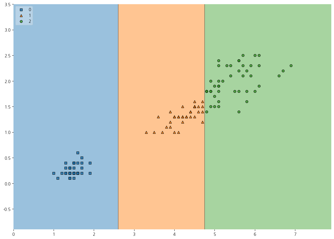
7-8. Testset의 예측결과에 대한 시각화해보기
plt.figure(figsize=(14,10))
plot_decision_regions(X=X_test, y=y_pred, clf=dt, legend=2)
plt.show()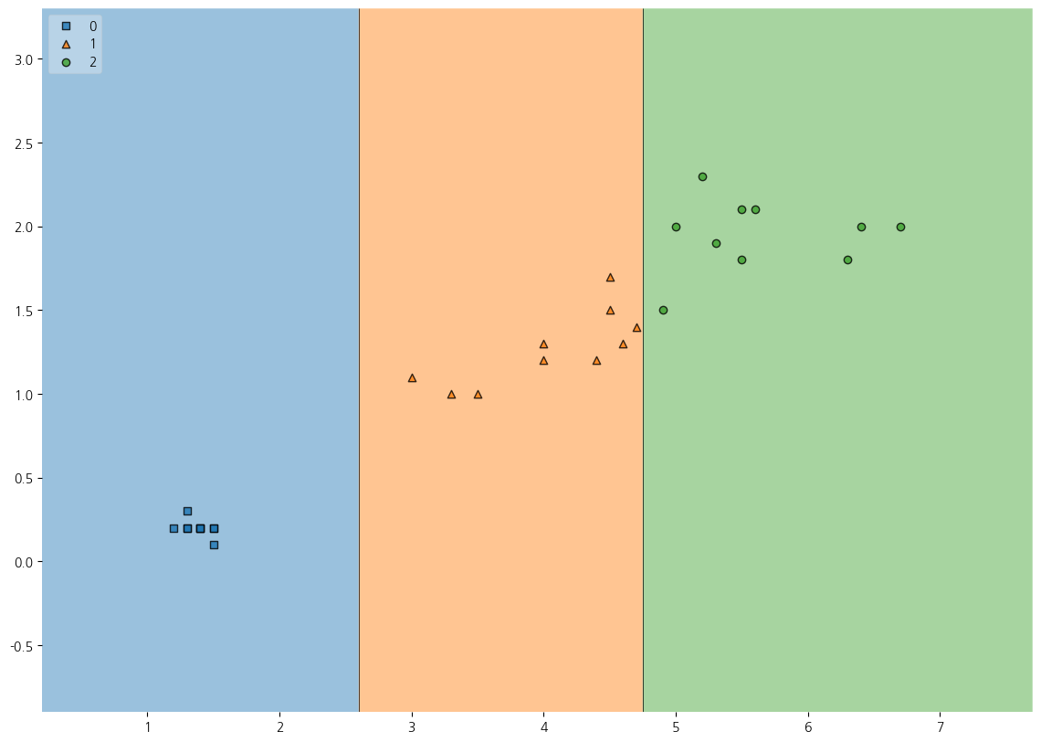
CH1-07(2) 전체 feature을 사용하여 Decision Tree로 Iris데이터셋 예측하기
from sklearn.tree import DecisionTreeClassifier
from sklearn.model_selection import train_test_split
from sklearn.metrics import accuracy_score
from sklearn.metrics import roc_auc_score
from mlxtend.plotting import plot_decision_regions
import pandas as pd
import numpy as np
import matplotlib.pyplot as plt
import koreanize_matplotlib
import seaborn as snsX_train, X_test, y_train, y_test = train_test_split(X,y,test_size=0.2,
stratify=y,random_state=2024)7-1. 전체 피처를 사용하여 예측해 보았더니 test accuracy가 0.96666이고 train accuracy가 0.99166정도
dt_clf = DecisionTreeClassifier(max_depth=5, random_state=2024)
dt_clf.fit(X_train,y_train)
print(dt_clf.score(X_test,y_test))0.9666666666666667y_train_pred = dt_clf.predict(X_train)
print(accuracy_score(y_train, y_train_pred))0.99166666666666677-2. 방금 학습한 DecisionTree 모델을 사용하여 임의의 피처 값에 대해 예측해보자
tmp_data = np.array([[2, 1.5, 2, 3.3]])
dt_clf.predict(tmp_data)array([1])dt_clf.predict_proba(tmp_data)array([[0., 1., 0.]])dt_clf.classes_array([0, 1, 2])7-3. 특성중요도
dt_clf.feature_importances_array([0. , 0.01694915, 0.42021683, 0.56283402])feature_importances = dict(zip(iris_raw.feature_names, dt_clf.feature_importances_))
feature_importances{'sepal length (cm)': 0.0,
'sepal width (cm)': 0.016949152542372878,
'petal length (cm)': 0.42021682699648794,
'petal width (cm)': 0.5628340204611392}CH1-08: zip과 언패킹인자
8-1. 튜플을 dict로
pairs = ('a',1), ('b',2), ('c',3)
dict(pairs)
{'a': 1, 'b': 2, 'c': 3}a = list(zip(*pairs))
b = list(a[0])
c = list(a[1])
print(b, c)['a', 'b', 'c'] [1, 2, 3]CH2-01~CH2-03. 타이타닉 생존자 예측
1-01. Data SET 불러오고 살펴보기
titanic_df = pd.read_excel('../titanic/titanic.xls')titanic_df.head()| pclass | survived | name | sex | age | sibsp | parch | ticket | fare | cabin | embarked | boat | body | home.dest | |
|---|---|---|---|---|---|---|---|---|---|---|---|---|---|---|
| 0 | 1 | 1 | Allen, Miss. Elisabeth Walton | female | 29.0000 | 0 | 0 | 24160 | 211.3375 | B5 | S | 2 | NaN | St Louis, MO |
| 1 | 1 | 1 | Allison, Master. Hudson Trevor | male | 0.9167 | 1 | 2 | 113781 | 151.5500 | C22 C26 | S | 11 | NaN | Montreal, PQ / Chesterville, ON |
| 2 | 1 | 0 | Allison, Miss. Helen Loraine | female | 2.0000 | 1 | 2 | 113781 | 151.5500 | C22 C26 | S | NaN | NaN | Montreal, PQ / Chesterville, ON |
| 3 | 1 | 0 | Allison, Mr. Hudson Joshua Creighton | male | 30.0000 | 1 | 2 | 113781 | 151.5500 | C22 C26 | S | NaN | 135.0 | Montreal, PQ / Chesterville, ON |
| 4 | 1 | 0 | Allison, Mrs. Hudson J C (Bessie Waldo Daniels) | female | 25.0000 | 1 | 2 | 113781 | 151.5500 | C22 C26 | S | NaN | NaN | Montreal, PQ / Chesterville, ON |
titanic_df.info()<class 'pandas.core.frame.DataFrame'>
RangeIndex: 1309 entries, 0 to 1308
Data columns (total 14 columns):
# Column Non-Null Count Dtype
--- ------ -------------- -----
0 pclass 1309 non-null int64
1 survived 1309 non-null int64
2 name 1309 non-null object
3 sex 1309 non-null object
4 age 1046 non-null float64
5 sibsp 1309 non-null int64
6 parch 1309 non-null int64
7 ticket 1309 non-null object
8 fare 1308 non-null float64
9 cabin 295 non-null object
10 embarked 1307 non-null object
11 boat 486 non-null object
12 body 121 non-null float64
13 home.dest 745 non-null object
dtypes: float64(3), int64(4), object(7)
memory usage: 143.3+ KBtitanic_df.describe(exclude='object')| pclass | survived | age | sibsp | parch | fare | body | |
|---|---|---|---|---|---|---|---|
| count | 1309.000000 | 1309.000000 | 1046.000000 | 1309.000000 | 1309.000000 | 1308.000000 | 121.000000 |
| mean | 2.294882 | 0.381971 | 29.881135 | 0.498854 | 0.385027 | 33.295479 | 160.809917 |
| std | 0.837836 | 0.486055 | 14.413500 | 1.041658 | 0.865560 | 51.758668 | 97.696922 |
| min | 1.000000 | 0.000000 | 0.166700 | 0.000000 | 0.000000 | 0.000000 | 1.000000 |
| 25% | 2.000000 | 0.000000 | 21.000000 | 0.000000 | 0.000000 | 7.895800 | 72.000000 |
| 50% | 3.000000 | 0.000000 | 28.000000 | 0.000000 | 0.000000 | 14.454200 | 155.000000 |
| 75% | 3.000000 | 1.000000 | 39.000000 | 1.000000 | 0.000000 | 31.275000 | 256.000000 |
| max | 3.000000 | 1.000000 | 80.000000 | 8.000000 | 9.000000 | 512.329200 | 328.000000 |
titanic_df.describe(exclude='number')| name | sex | ticket | cabin | embarked | boat | home.dest | |
|---|---|---|---|---|---|---|---|
| count | 1309 | 1309 | 1309 | 295 | 1307 | 486 | 745 |
| unique | 1307 | 2 | 939 | 186 | 3 | 28 | 369 |
| top | Connolly, Miss. Kate | male | CA. 2343 | C23 C25 C27 | S | 13 | New York, NY |
| freq | 2 | 843 | 11 | 6 | 914 | 39 | 64 |
1-2. 성별 생존율 pie plot으로 시각화해보기
survival_cnt = titanic_df['survived'].value_counts()
sex_cnt = titanic_df['sex'].value_counts()
fig, ax = plt.subplots(1,2, figsize=(20,13))
ax[0].pie(survival_cnt, autopct = '%1.1f%%', explode = [0, 0.05],
          labels=['Not Survived','Survived']);
sns.countplot(data=titanic_df, x='survived',hue='sex',ax=ax[1])<Axes: xlabel='survived', ylabel='count'>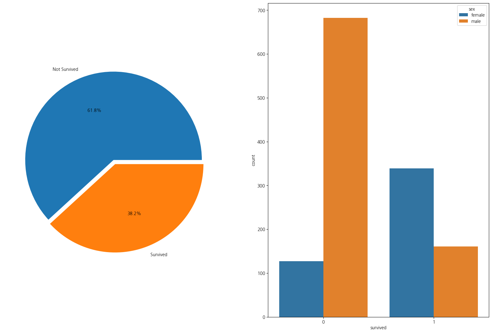
1-3. 성별 탑승자수와 성별에 따른 생존
import numpy as np
fig, ax = plt.subplots(1,2, figsize=(20,12))
sns.countplot(data=titanic_df, x='sex',ax=ax[0])
sns.countplot(data=titanic_df,x='sex',hue='survived',ax=ax[1])
plt.show();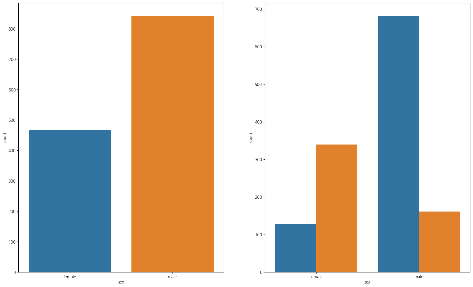
1-4. 경제력과 생존율
- 보면 1등석이 가장 생존율이 높음을 알 수 있다
pd.crosstab(titanic_df['pclass'], titanic_df['survived'], margins=True)| survived | 0 | 1 | All |
|---|---|---|---|
| pclass | |||
| 1 | 123 | 200 | 323 |
| 2 | 158 | 119 | 277 |
| 3 | 528 | 181 | 709 |
| All | 809 | 500 | 1309 |
1-5. 나이와 pclass(선실등급)별 생존인원 수
- 선실등급이 높을수록 생존확률이 높음
grid = sns.FacetGrid(titanic_df, row='pclass',col='survived', height=4, aspect=2,dropna=True)
grid.map(plt.hist, 'age',alpha=0.5,bins=20)
grid.add_legend();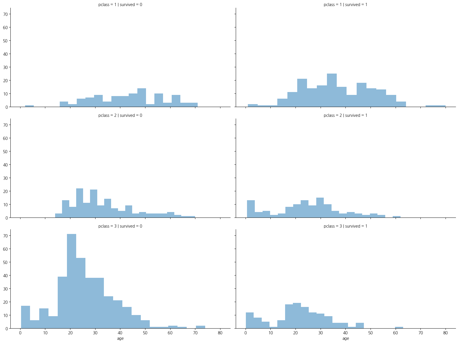
1-6. 나이를 5단계로 분할하기(pd.cut)
titanic_df['age_bin'] = pd.cut(titanic_df['age'], bins = [0,7,15,30,60,100],
                            include_lowest=True, labels=['baby','teen','young',
                                                         'adult','old'])
titanic_df.head()| pclass | survived | name | sex | age | sibsp | parch | ticket | fare | cabin | embarked | boat | body | home.dest | age_bin | |
|---|---|---|---|---|---|---|---|---|---|---|---|---|---|---|---|
| 0 | 1 | 1 | Allen, Miss. Elisabeth Walton | female | 29.0000 | 0 | 0 | 24160 | 211.3375 | B5 | S | 2 | NaN | St Louis, MO | young |
| 1 | 1 | 1 | Allison, Master. Hudson Trevor | male | 0.9167 | 1 | 2 | 113781 | 151.5500 | C22 C26 | S | 11 | NaN | Montreal, PQ / Chesterville, ON | baby |
| 2 | 1 | 0 | Allison, Miss. Helen Loraine | female | 2.0000 | 1 | 2 | 113781 | 151.5500 | C22 C26 | S | NaN | NaN | Montreal, PQ / Chesterville, ON | baby |
| 3 | 1 | 0 | Allison, Mr. Hudson Joshua Creighton | male | 30.0000 | 1 | 2 | 113781 | 151.5500 | C22 C26 | S | NaN | 135.0 | Montreal, PQ / Chesterville, ON | young |
| 4 | 1 | 0 | Allison, Mrs. Hudson J C (Bessie Waldo Daniels) | female | 25.0000 | 1 | 2 | 113781 | 151.5500 | C22 C26 | S | NaN | NaN | Montreal, PQ / Chesterville, ON | young |
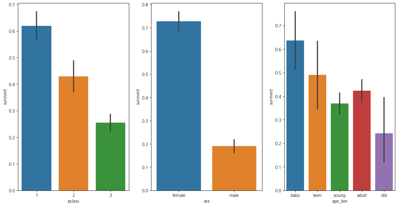
1-7. 나이 성별 선실등급별 생존율 한번에 확인하기
plt.figure(figsize=(16,8))
plt.subplot(131)
sns.barplot(data=titanic_df, x='pclass',y='survived')
plt.subplot(132)
sns.barplot(data=titanic_df, x='sex', y='survived')
plt.subplot(133)
sns.barplot(data=titanic_df, x='age_bin', y='survived')
plt.show()
C:\Users\kd010\miniconda3\Lib\site-packages\seaborn\categorical.py:641: FutureWarning: The default of observed=False is deprecated and will be changed to True in a future version of pandas. Pass observed=False to retain current behavior or observed=True to adopt the future default and silence this warning.
grouped_vals = vals.groupby(grouper)