CH2-04 타이타닉 분석 EDA3(참고사항: survived칼럼에서 양의클래스인 1이 생존, 음의클래스인 0이 사망임)
import sklearn
import pandas as pd
import numpy as np
import matplotlib.pyplot as plt
import koreanize_matplotlib
import seaborn as sns
titanic_df = pd.read_excel('../titanic/titanic.xls')
titanic_df| pclass | survived | name | sex | age | sibsp | parch | ticket | fare | cabin | embarked | boat | body | home.dest | |
|---|---|---|---|---|---|---|---|---|---|---|---|---|---|---|
| 0 | 1 | 1 | Allen, Miss. Elisabeth Walton | female | 29.0000 | 0 | 0 | 24160 | 211.3375 | B5 | S | 2 | NaN | St Louis, MO |
| 1 | 1 | 1 | Allison, Master. Hudson Trevor | male | 0.9167 | 1 | 2 | 113781 | 151.5500 | C22 C26 | S | 11 | NaN | Montreal, PQ / Chesterville, ON |
| 2 | 1 | 0 | Allison, Miss. Helen Loraine | female | 2.0000 | 1 | 2 | 113781 | 151.5500 | C22 C26 | S | NaN | NaN | Montreal, PQ / Chesterville, ON |
| 3 | 1 | 0 | Allison, Mr. Hudson Joshua Creighton | male | 30.0000 | 1 | 2 | 113781 | 151.5500 | C22 C26 | S | NaN | 135.0 | Montreal, PQ / Chesterville, ON |
| 4 | 1 | 0 | Allison, Mrs. Hudson J C (Bessie Waldo Daniels) | female | 25.0000 | 1 | 2 | 113781 | 151.5500 | C22 C26 | S | NaN | NaN | Montreal, PQ / Chesterville, ON |
| ... | ... | ... | ... | ... | ... | ... | ... | ... | ... | ... | ... | ... | ... | ... |
| 1304 | 3 | 0 | Zabour, Miss. Hileni | female | 14.5000 | 1 | 0 | 2665 | 14.4542 | NaN | C | NaN | 328.0 | NaN |
| 1305 | 3 | 0 | Zabour, Miss. Thamine | female | NaN | 1 | 0 | 2665 | 14.4542 | NaN | C | NaN | NaN | NaN |
| 1306 | 3 | 0 | Zakarian, Mr. Mapriededer | male | 26.5000 | 0 | 0 | 2656 | 7.2250 | NaN | C | NaN | 304.0 | NaN |
| 1307 | 3 | 0 | Zakarian, Mr. Ortin | male | 27.0000 | 0 | 0 | 2670 | 7.2250 | NaN | C | NaN | NaN | NaN |
| 1308 | 3 | 0 | Zimmerman, Mr. Leo | male | 29.0000 | 0 | 0 | 315082 | 7.8750 | NaN | S | NaN | NaN | NaN |
1309 rows × 14 columns
titanic_df.info()<class 'pandas.core.frame.DataFrame'>
RangeIndex: 1309 entries, 0 to 1308
Data columns (total 14 columns):
# Column Non-Null Count Dtype
--- ------ -------------- -----
0 pclass 1309 non-null int64
1 survived 1309 non-null int64
2 name 1309 non-null object
3 sex 1309 non-null object
4 age 1046 non-null float64
5 sibsp 1309 non-null int64
6 parch 1309 non-null int64
7 ticket 1309 non-null object
8 fare 1308 non-null float64
9 cabin 295 non-null object
10 embarked 1307 non-null object
11 boat 486 non-null object
12 body 121 non-null float64
13 home.dest 745 non-null object
dtypes: float64(3), int64(4), object(7)
memory usage: 143.3+ KB1-1. 남녀별 연령에 따른 생존인원 시각화해보기
women = titanic_df.loc[titanic_df['sex'] == 'female',:]
men = titanic_df.loc[titanic_df['sex'] == 'male',:]
fig, axes = plt.subplots(1,2,figsize=(20,10))
sns.histplot(women, bins=40,x = 'age',hue='survived',ax=axes[0])
axes[0].set_title('number of survived women by age')
sns.histplot(men,bins=40,x='age',hue='survived',ax=axes[1])
axes[1].set_title('number of survived men by age')
plt.show()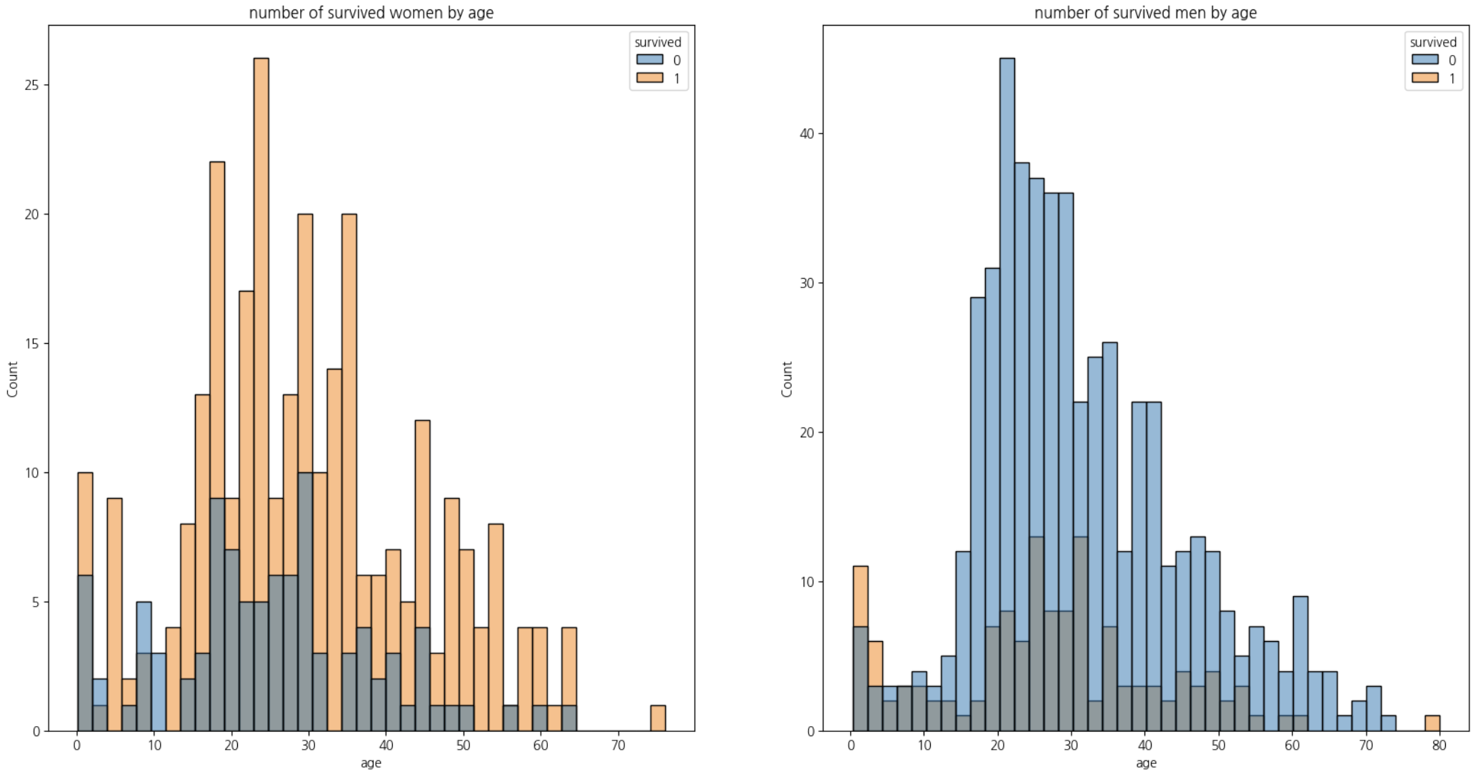
1-2. Name 칼럼에서 Title을 추출하여 Title 칼럼 추가하기
titanic_df.describe(exclude='number')| name | sex | ticket | cabin | embarked | boat | home.dest | |
|---|---|---|---|---|---|---|---|
| count | 1309 | 1309 | 1309 | 295 | 1307 | 486 | 745 |
| unique | 1307 | 2 | 939 | 186 | 3 | 28 | 369 |
| top | Connolly, Miss. Kate | male | CA. 2343 | C23 C25 C27 | S | 13 | New York, NY |
| freq | 2 | 843 | 11 | 6 | 914 | 39 | 64 |
titanic_df['title'] = titanic_df['name'].apply(lambda x: x.split(',')[1].split('.')[0].strip())
titanic_df.head()| pclass | survived | name | sex | age | sibsp | parch | ticket | fare | cabin | embarked | boat | body | home.dest | title | |
|---|---|---|---|---|---|---|---|---|---|---|---|---|---|---|---|
| 0 | 1 | 1 | Allen, Miss. Elisabeth Walton | female | 29.0000 | 0 | 0 | 24160 | 211.3375 | B5 | S | 2 | NaN | St Louis, MO | Miss |
| 1 | 1 | 1 | Allison, Master. Hudson Trevor | male | 0.9167 | 1 | 2 | 113781 | 151.5500 | C22 C26 | S | 11 | NaN | Montreal, PQ / Chesterville, ON | Master |
| 2 | 1 | 0 | Allison, Miss. Helen Loraine | female | 2.0000 | 1 | 2 | 113781 | 151.5500 | C22 C26 | S | NaN | NaN | Montreal, PQ / Chesterville, ON | Miss |
| 3 | 1 | 0 | Allison, Mr. Hudson Joshua Creighton | male | 30.0000 | 1 | 2 | 113781 | 151.5500 | C22 C26 | S | NaN | 135.0 | Montreal, PQ / Chesterville, ON | Mr |
| 4 | 1 | 0 | Allison, Mrs. Hudson J C (Bessie Waldo Daniels) | female | 25.0000 | 1 | 2 | 113781 | 151.5500 | C22 C26 | S | NaN | NaN | Montreal, PQ / Chesterville, ON | Mrs |
1-3. title의 성별 분포 보기
pd.crosstab(index=titanic_df['title'],columns=titanic_df['sex'])| sex | female | male |
|---|---|---|
| title | ||
| Capt | 0 | 1 |
| Col | 0 | 4 |
| Don | 0 | 1 |
| Dona | 1 | 0 |
| Dr | 1 | 7 |
| Jonkheer | 0 | 1 |
| Lady | 1 | 0 |
| Major | 0 | 2 |
| Master | 0 | 61 |
| Miss | 260 | 0 |
| Mlle | 2 | 0 |
| Mme | 1 | 0 |
| Mr | 0 | 757 |
| Mrs | 197 | 0 |
| Ms | 2 | 0 |
| Rev | 0 | 8 |
| Sir | 0 | 1 |
| the Countess | 1 | 0 |
1-4. title 분류하기
남성의 호칭:
Mr: 일반적인 성인 남성의 호칭.
Master: 주로 미혼 남성 아동에게 사용되는 호칭.
Sir: 기사(Knight)에게 주어지는 호칭, 하지만 여기서는 아마도 존경을 표하는 의미로 사용될 수 있습니다.
여성의 호칭:
Miss: 미혼 여성.
Mrs: 기혼 여성.
Ms: 결혼 여부에 관계없이 여성에게 사용할 수 있는 호칭.
Mlle: 프랑스어로 ‘마드모아젤(Mademoiselle)’, 미혼 여성에게 사용되는 호칭, Miss와 같은 의미.
Mme: 프랑스어로 ‘마담(Madame)’, 기혼 여성에게 사용되는 호칭, Mrs와 같은 의미.
Lady: 귀족 여성의 호칭, 특정 문화에서는 기혼 여성에게도 사용될 수 있습니다.
Dona: 스페인어 및 포르투갈어권 국가에서 사용되는 여성 호칭, ‘Lady’나 ‘Madam’과 유사한 존경을 표하는 호칭.
the Countess: 백작 부인의 호칭.
군사 및 전문 직업 호칭:
Col: 대령.
Major: 소령.
Capt: 대위, 해군에서는 대령에 해당할 수 있음.
Dr: 의사나 박사학위를 가진 사람.
Rev: 목사, 신부 등의 종교 지도자.
기타 특별 호칭:
Jonkheer: 네덜란드의 낮은 귀족 호칭.
Don: 스페인어권 국가에서 남성에게 사용되는 존경을 표하는 호칭.
비슷한 의미를 가지는 호칭을 정리하면:
Miss와 Mlle은 미혼 여성을 의미합니다.
Mrs와 Mme은 기혼 여성을 의미합니다.
Ms는 결혼 여부에 관계없이 여성에게 사용될 수 있으며, 현대적인 호칭으로 여겨집니다.
Lady와 Dona, the Countess는 모두 존경을 표하는 여성 호칭
으로, 귀족이나 높은 사회적 지위의 여성에게 사용됩니다.
titanic_df['title'] = titanic_df['title'].replace('Mme','Miss').replace('Mlle','Miss').replace('Ms','Miss')titanic_df['title'].unique()array(['Miss', 'Master', 'Mr', 'Mrs', 'Col', 'Dr', 'Major', 'Capt',
'Lady', 'Sir', 'Dona', 'Jonkheer', 'the Countess', 'Don', 'Rev'],
dtype=object)1-5. 귀족이나 전문직 나타내는 호칭 정리하기
rare_f = ['Lady','Dona','the Countess']
rare_m = ['Dr','Jonkheer','Don','Col','Major','Capt','Rev','Sir']
titanic_df['title'] = titanic_df['title'].replace(rare_f,'rare_f').replace(rare_m,'rare_m')
titanic_df['title'].unique()
array(['Miss', 'Master', 'Mr', 'Mrs', 'rare_m', 'rare_f'], dtype=object)titanic_df['title'].value_counts(ascending=True)title
rare_f 3
rare_m 26
Master 61
Mrs 197
Miss 265
Mr 757
Name: count, dtype: int641-6. title에 따른 생존율 살펴보기
- rare_f(여자 귀족, 전문직)의 생존율은 매우 높고,
- 여자에 rare_m는 아까 rare_m으로 분류했던 'Dr'중 여성이 한 명 있어서 그렇고
- 남자의 rare_m(남자 귀족, 전문직)의 생존율은 'Mr'(성인 남성)보다는 높으나 'Master'(미혼 남성 아동)보다는 낮음
titanic_df.groupby(['sex','title'])[['survived']].agg('mean')| survived | ||
|---|---|---|
| sex | title | |
| female | Miss | 0.679245 |
| Mrs | 0.786802 | |
| rare_f | 1.000000 | |
| rare_m | 1.000000 | |
| male | Master | 0.508197 |
| Mr | 0.162483 | |
| rare_m | 0.280000 |
CH2-06: 타이타닉 머신러닝 모델 구축
라벨 인코딩(Label Encoding)
라벨 인코딩은 범주형 변수의 각 범주를 숫자 값으로 변환합니다. 예를 들어, '성별' 칼럼에 'male'과 'female'이 있다면, 'male'은 0으로, 'female'은 1로 매핑할 수 있습니다.
장점:
모델 입력을 위해 데이터의 차원을 증가시키지 않습니다.
트리 기반 모델(예: 결정 트리, 랜덤 포레스트)에서 잘 작동할 수 있습니다.
단점:
숫자 값에 순서나 중요도가 있는 것처럼 해석될 수 있어, 선형 모델(예: 선형 회귀, 로지스틱 회귀)에서 잘못된 관계를 학습할 수 있습니다.
원-핫 인코딩(One-Hot Encoding)
원-핫 인코딩은 범주형 변수의 각 범주를 독립된 이진 특성으로 변환합니다. '성별' 칼럼의 경우, 'male'과 'female'은 두 개의 칼럼으로 변환되며, 각각의 칼럼은 해당 성별일 때 1, 아닐 때 0의 값을 가집니다.
장점:
선형 모델에서 범주 간에 순서나 중요도를 부여하지 않으므로 더 적합할 수 있습니다.
모델이 범주형 변수의 각 범주를 독립적으로 처리할 수 있게 해줍니다.
단점:
데이터셋의 특성 수를 증가시킵니다. 많은 범주를 가진 변수에 대해 원-핫 인코딩을 수행하면 차원의 저주로 인해 모델 성능이 저하될 수 있습니다.
결정 요소
모델 종류: 트리 기반 모델을 사용한다면 라벨 인코딩이 더 적합할 수 있습니다. 선형 모델이나 신경망을 사용한다면 원-핫 인코딩이 더 적합할 수 있습니다.
데이터의 특성: '성별'과 같이 범주가 명확하고, 두 개뿐인 경우 원-핫 인코딩을 사용하는 것이 일반적으로 안전합니다. 이는 모델이 성별이라는 특성을 더 명확하게 구분할 수 있게 해주기 때문입니다.
1-1. 라벨인코딩 하기
from sklearn.preprocessing import LabelEncoder
lb = LabelEncoder()
titanic_df['gender'] = lb.fit_transform(titanic_df['sex'])titanic_df['gender'].value_counts()gender
1 843
0 466
Name: count, dtype: int641-3. 결측치 확인 및 결측치 대체
titanic_df.info()<class 'pandas.core.frame.DataFrame'>
RangeIndex: 1309 entries, 0 to 1308
Data columns (total 16 columns):
# Column Non-Null Count Dtype
--- ------ -------------- -----
0 pclass 1309 non-null int64
1 survived 1309 non-null int64
2 name 1309 non-null object
3 sex 1309 non-null object
4 age 1046 non-null float64
5 sibsp 1309 non-null int64
6 parch 1309 non-null int64
7 ticket 1309 non-null object
8 fare 1308 non-null float64
9 cabin 295 non-null object
10 embarked 1307 non-null object
11 boat 486 non-null object
12 body 121 non-null float64
13 home.dest 745 non-null object
14 title 1309 non-null object
15 gender 1309 non-null int32
dtypes: float64(3), int32(1), int64(4), object(8)
memory usage: 158.6+ KBtitanic_df[0:891].info()<class 'pandas.core.frame.DataFrame'>
RangeIndex: 891 entries, 0 to 890
Data columns (total 16 columns):
# Column Non-Null Count Dtype
--- ------ -------------- -----
0 pclass 891 non-null int64
1 survived 891 non-null int64
2 name 891 non-null object
3 sex 891 non-null object
4 age 795 non-null float64
5 sibsp 891 non-null int64
6 parch 891 non-null int64
7 ticket 891 non-null object
8 fare 891 non-null float64
9 cabin 281 non-null object
10 embarked 889 non-null object
11 boat 386 non-null object
12 body 88 non-null float64
13 home.dest 742 non-null object
14 title 891 non-null object
15 gender 891 non-null int32
dtypes: float64(3), int32(1), int64(4), object(8)
memory usage: 108.0+ KB1-4. 일단 결측치가 50%넘어가는 cabin,boat,body 없애고 다시 age_cat 만들어주기
titanic_df = titanic_df.drop(columns=['cabin','boat','body'], axis=1)titanic_df.info()<class 'pandas.core.frame.DataFrame'>
RangeIndex: 1309 entries, 0 to 1308
Data columns (total 13 columns):
# Column Non-Null Count Dtype
--- ------ -------------- -----
0 pclass 1309 non-null int64
1 survived 1309 non-null int64
2 name 1309 non-null object
3 sex 1309 non-null object
4 age 1046 non-null float64
5 sibsp 1309 non-null int64
6 parch 1309 non-null int64
7 ticket 1309 non-null object
8 fare 1308 non-null float64
9 embarked 1307 non-null object
10 home.dest 745 non-null object
11 title 1309 non-null object
12 gender 1309 non-null int32
dtypes: float64(2), int32(1), int64(4), object(6)
memory usage: 128.0+ KB1-5 train데이터의 title별 age의 중앙값 살펴보고 age와 age_cat의 결측치를 이걸로 대체하기
train.groupby('title')[['age']].agg('median')| age | |
|---|---|
| title | |
| Master | 3.5 |
| Miss | 22.0 |
| Mr | 30.0 |
| Mrs | 36.0 |
| rare_f | 39.0 |
| rare_m | 49.0 |
def fill_age(dataframe):
    dataframe.loc[titanic_df['title'] == 'Master','age']=dataframe.loc[titanic_df['title'] == 'Master','age'].fillna(3.5)
    dataframe.loc[titanic_df['title'] == 'Miss','age']=dataframe.loc[titanic_df['title'] == 'Miss','age'].fillna(22.0)
    dataframe.loc[titanic_df['title'] == 'Mr','age']=dataframe.loc[titanic_df['title'] == 'Mr','age'].fillna(30.0)
    dataframe.loc[titanic_df['title'] == 'Mrs','age']=dataframe.loc[titanic_df['title'] == 'Mrs','age'].fillna(36.0)
    dataframe.loc[titanic_df['title'] == 'rare_f','age']=dataframe.loc[titanic_df['title'] == 'rare_f','age'].fillna(39.0)
    dataframe.loc[titanic_df['title'] == 'rare_m','age']=dataframe.loc[titanic_df['title'] == 'rare_m','age'].fillna(49.0)

    return dataframe

def age_bin(dataframe):
    dataframe['age_bin'] = pd.cut(titanic_df['age'], bins = [0,7,15,30,60,100],
                            include_lowest=True, labels=['baby','teen','young',
                                                         'adult','old'])
    return dataframe
titanic_df = fill_age(titanic_df)
titanic_df = age_bin(titanic_df)
titanic_df.info()<class 'pandas.core.frame.DataFrame'>
RangeIndex: 1309 entries, 0 to 1308
Data columns (total 14 columns):
# Column Non-Null Count Dtype
--- ------ -------------- -----
0 pclass 1309 non-null int64
1 survived 1309 non-null int64
2 name 1309 non-null object
3 sex 1309 non-null object
4 age 1309 non-null float64
5 sibsp 1309 non-null int64
6 parch 1309 non-null int64
7 ticket 1309 non-null object
8 fare 1308 non-null float64
9 embarked 1307 non-null object
10 home.dest 745 non-null object
11 title 1309 non-null object
12 gender 1309 non-null int32
13 age_bin 1309 non-null category
dtypes: category(1), float64(2), int32(1), int64(4), object(6)
memory usage: 129.4+ KB1-6. home.dest 분석
- 아무래도 고유값이 369라 별 의미가 없을거 같아 드랍
titanic_df = titanic_df.drop(columns='home.dest',axis=1)titanic_df.info()<class 'pandas.core.frame.DataFrame'>
RangeIndex: 1309 entries, 0 to 1308
Data columns (total 13 columns):
# Column Non-Null Count Dtype
--- ------ -------------- -----
0 pclass 1309 non-null int64
1 survived 1309 non-null int64
2 name 1309 non-null object
3 sex 1309 non-null object
4 age 1309 non-null float64
5 sibsp 1309 non-null int64
6 parch 1309 non-null int64
7 ticket 1309 non-null object
8 fare 1308 non-null float64
9 embarked 1307 non-null object
10 title 1309 non-null object
11 gender 1309 non-null int32
12 age_bin 1309 non-null category
dtypes: category(1), float64(2), int32(1), int64(4), object(5)
memory usage: 119.2+ KB1-7. 머신러닝 모델 만들기
titanic = titanic_df.drop(columns=['sex','name','ticket'])titanic| pclass | survived | age | sibsp | parch | fare | embarked | title | gender | age_bin | |
|---|---|---|---|---|---|---|---|---|---|---|
| 0 | 1 | 1 | 29.0000 | 0 | 0 | 211.3375 | S | Miss | 0 | young |
| 1 | 1 | 1 | 0.9167 | 1 | 2 | 151.5500 | S | Master | 1 | baby |
| 2 | 1 | 0 | 2.0000 | 1 | 2 | 151.5500 | S | Miss | 0 | baby |
| 3 | 1 | 0 | 30.0000 | 1 | 2 | 151.5500 | S | Mr | 1 | young |
| 4 | 1 | 0 | 25.0000 | 1 | 2 | 151.5500 | S | Mrs | 0 | young |
| ... | ... | ... | ... | ... | ... | ... | ... | ... | ... | ... |
| 1304 | 3 | 0 | 14.5000 | 1 | 0 | 14.4542 | C | Miss | 0 | teen |
| 1305 | 3 | 0 | 22.0000 | 1 | 0 | 14.4542 | C | Miss | 0 | young |
| 1306 | 3 | 0 | 26.5000 | 0 | 0 | 7.2250 | C | Mr | 1 | young |
| 1307 | 3 | 0 | 27.0000 | 0 | 0 | 7.2250 | C | Mr | 1 | young |
| 1308 | 3 | 0 | 29.0000 | 0 | 0 | 7.8750 | S | Mr | 1 | young |
1309 rows × 10 columns
titanic['embarked'] = le.fit_transform(titanic['embarked'])
titanic['title'] = le.fit_transform(titanic['title'])
titanic['age_bin'] = le.fit_transform(titanic['age_bin'])titanic| pclass | survived | age | sibsp | parch | fare | embarked | title | gender | age_bin | |
|---|---|---|---|---|---|---|---|---|---|---|
| 0 | 1 | 1 | 29.0000 | 0 | 0 | 211.3375 | 2 | 1 | 0 | 4 |
| 1 | 1 | 1 | 0.9167 | 1 | 2 | 151.5500 | 2 | 0 | 1 | 1 |
| 2 | 1 | 0 | 2.0000 | 1 | 2 | 151.5500 | 2 | 1 | 0 | 1 |
| 3 | 1 | 0 | 30.0000 | 1 | 2 | 151.5500 | 2 | 2 | 1 | 4 |
| 4 | 1 | 0 | 25.0000 | 1 | 2 | 151.5500 | 2 | 3 | 0 | 4 |
| ... | ... | ... | ... | ... | ... | ... | ... | ... | ... | ... |
| 1304 | 3 | 0 | 14.5000 | 1 | 0 | 14.4542 | 0 | 1 | 0 | 3 |
| 1305 | 3 | 0 | 22.0000 | 1 | 0 | 14.4542 | 0 | 1 | 0 | 4 |
| 1306 | 3 | 0 | 26.5000 | 0 | 0 | 7.2250 | 0 | 2 | 1 | 4 |
| 1307 | 3 | 0 | 27.0000 | 0 | 0 | 7.2250 | 0 | 2 | 1 | 4 |
| 1308 | 3 | 0 | 29.0000 | 0 | 0 | 7.8750 | 2 | 2 | 1 | 4 |
1309 rows × 10 columns
titanic.loc[titanic['fare'].isna(),:]| pclass | survived | age | sibsp | parch | fare | embarked | title | gender | age_bin | |
|---|---|---|---|---|---|---|---|---|---|---|
| 1225 | 3 | 0 | 60.5 | 0 | 0 | NaN | 2 | 2 | 1 | 2 |
titanic.dropna(axis=0,inplace=True)titanic.info()<class 'pandas.core.frame.DataFrame'>
Index: 1308 entries, 0 to 1308
Data columns (total 10 columns):
# Column Non-Null Count Dtype
--- ------ -------------- -----
0 pclass 1308 non-null int64
1 survived 1308 non-null int64
2 age 1308 non-null float64
3 sibsp 1308 non-null int64
4 parch 1308 non-null int64
5 fare 1308 non-null float64
6 embarked 1308 non-null int32
7 title 1308 non-null int32
8 gender 1308 non-null int32
9 age_bin 1308 non-null int32
dtypes: float64(2), int32(4), int64(4)
memory usage: 92.0 KBX = titanic.drop(columns='survived',axis=1)
y = titanic['survived']from sklearn.model_selection import train_test_split
X_train,X_test,y_train,y_test = train_test_split(X,y, stratify=y, test_size=0.2, random_state=42)print(X_train.shape,y_train.shape,X_test.shape, y_test.shape)(1046, 9) (1046,) (262, 9) (262,)from sklearn.ensemble import RandomForestClassifier1-8. 머신러닝 예측 결과 분석
rf = RandomForestClassifier(n_estimators=100,criterion='entropy',max_depth=10,n_jobs=-1)
rf.fit(X_train,y_train)
rf.score(X_test,y_test)0.8435114503816794y_pred = rf.predict(X_test)from sklearn.metrics import confusion_matrix,classification_reportconfusion_matrix(y_test, y_pred)array([[144, 18],
[ 23, 77]], dtype=int64)print(classification_report(y_test, y_pred)) precision recall f1-score support
0 0.86 0.89 0.88 162
1 0.81 0.77 0.79 100
accuracy 0.84 262
macro avg 0.84 0.83 0.83 262
weighted avg 0.84 0.84 0.84 2621-9. test 데이터의 각 샘플의 생존확률예측 데이터프레임 보기(1이 생존, 0이 사망)
prob = rf.predict_proba(X_test)
prob_df = pd.DataFrame(prob)
prob_df.head()| 0 | 1 | |
|---|---|---|
| 0 | 0.494642 | 0.505358 |
| 1 | 0.273222 | 0.726778 |
| 2 | 0.872152 | 0.127848 |
| 3 | 0.826092 | 0.173908 |
| 4 | 0.931497 | 0.068503 |
1-10. 특성중요도 시각화
feature_imp = pd.DataFrame({'feature':X.columns, 'feature_imp':rf.feature_importances_})feature_imp.sort_values(by='feature_imp', ascending=False).reset_index(drop=True)| feature | feature_imp | |
|---|---|---|
| 0 | fare | 0.239013 |
| 1 | gender | 0.206034 |
| 2 | age | 0.186020 |
| 3 | title | 0.108987 |
| 4 | pclass | 0.094071 |
| 5 | sibsp | 0.058823 |
| 6 | parch | 0.040308 |
| 7 | embarked | 0.038364 |
| 8 | age_bin | 0.028381 |
CH3-02:MinMaxScaling
from sklearn.preprocessing import MinMaxScaler
mms = MinMaxScaler()
import numpy as np
import pandas as pd
a = np.array([10,20,-10,0,25])
b = np.array([1,2,3,1,0])
df = pd.DataFrame({'a':a,'b':b})df.info()<class 'pandas.core.frame.DataFrame'>
RangeIndex: 5 entries, 0 to 4
Data columns (total 2 columns):
# Column Non-Null Count Dtype
--- ------ -------------- -----
0 a 5 non-null int32
1 b 5 non-null int32
dtypes: int32(2)
memory usage: 172.0 bytesdf_minmax = mms.fit_transform(df)df_minmaxarray([[0.57142857, 0.33333333],
[0.85714286, 0.66666667],
[0. , 1. ],
[0.28571429, 0.33333333],
[1. , 0. ]])mms.min_array([0.28571429, 0. ])mms.data_min_array([-10., 0.])mms.data_max_array([25., 3.])mms.data_range_array([35., 3.])CH3-03. StandardScaler:z분포(표준정규분포)형태로 만들어줌,(평균이 0, 표준편차가 1로)
z = (x - u) / s

where `u` is the mean of the training samples or zero if `with_mean=False`,
and `s` is the standard deviation of the training samples or one if
`with_std=False`.


```python
df| a | b | |
|---|---|---|
| 0 | 10 | 1 |
| 1 | 20 | 2 |
| 2 | -10 | 3 |
| 3 | 0 | 1 |
| 4 | 25 | 0 |
from sklearn.preprocessing import StandardScaler
ss = StandardScaler()
df_scaled = ss.fit_transform(df)df_scaledarray([[ 0.07808688, -0.39223227],
[ 0.85895569, 0.58834841],
[-1.48365074, 1.56892908],
[-0.70278193, -0.39223227],
[ 1.2493901 , -1.37281295]])ss.scale_array([12.80624847, 1.0198039 ])ss.mean_array([9. , 1.4])ss.feature_names_in_array(['a', 'b'], dtype=object)ss.n_features_in_2ss.var_array([164. , 1.04])ss.n_samples_seen_5CH3-04. Robust Scaler

df=pd.DataFrame({'A':[0.1,0.2,0.3,0.4,1,1.1,5]})
df| A | |
|---|---|
| 0 | 0.1 |
| 1 | 0.2 |
| 2 | 0.3 |
| 3 | 0.4 |
| 4 | 1.0 |
| 5 | 1.1 |
| 6 | 5.0 |
from sklearn.preprocessing import RobustScaler
rb = RobustScaler()
df_scaler = df.copy()
df_scaler['minmax'] = mms.fit_transform(df)
df_scaler['robust'] = rb.fit_transform(df)
df_scaler['standard'] = ss.fit_transform(df)df_scaler| A | minmax | robust | standard | |
|---|---|---|---|---|
| 0 | 0.1 | 0.000000 | -0.375 | -0.656747 |
| 1 | 0.2 | 0.020408 | -0.250 | -0.594623 |
| 2 | 0.3 | 0.040816 | -0.125 | -0.532498 |
| 3 | 0.4 | 0.061224 | 0.000 | -0.470373 |
| 4 | 1.0 | 0.183673 | 0.750 | -0.097625 |
| 5 | 1.1 | 0.204082 | 0.875 | -0.035500 |
| 6 | 5.0 | 1.000000 | 5.750 | 2.387365 |
robust scaler가 이상치의 영향을 가장 적게 받음을 알 수 있음
import matplotlib.pyplot as plt
import seaborn as snsplt.figure(figsize=(15,8))
sns.boxplot(data=df_scaler,orient='h')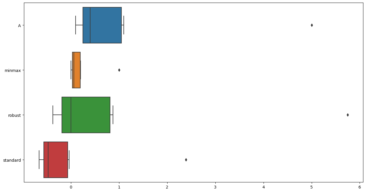
신경망에서 최소-최대 스케일링(MinMax Scaling)이 선호되는 주요 이유는 다음과 같습니다:
-
활성화 함수의 효율성: 많은 신경망의 활성화 함수, 특히 시그모이드(sigmoid)나 하이퍼볼릭 탄젠트(tanh)와 같은 함수들은 입력값이 작을 때 가장 잘 작동합니다. 이러한 함수들은 입력값이 특정 범위(시그모이드의 경우 0과 1 사이)에 있을 때 민감하게 반응하며, 너무 크거나 작은 값에 대해서는 포화(saturation)되어 기울기가 거의 0에 가까워질 수 있습니다. 최소-최대 스케일링은 모든 입력 값을 0과 1 사이로 맞춰줌으로써 이러한 활성화 함수들이 효율적으로 작동할 수 있는 환경을 만들어줍니다.
-
학습 속도 향상: 입력 데이터의 스케일이 비슷하면, 모델의 학습이 더 빠르게 수렴할 수 있습니다. 최소-최대 스케일링은 모든 특성 값을 동일한 범위로 조정함으로써, 가중치(weight)의 초기값에 대한 민감도를 줄이고 최적화 과정에서의 학습 속도를 향상시킬 수 있습니다.
-
그라디언트 소실 및 폭발 방지: 신경망에서는 그라디언트 기반 학습을 사용하기 때문에, 입력 값의 스케일이 너무 크거나 작으면 그라디언트 소실(vanishing gradients) 또는 폭발(exploding gradients) 문제가 발생할 수 있습니다. 최소-최대 스케일링을 통해 모든 입력 값을 일정 범위로 제한함으로써, 이러한 문제를 완화할 수 있습니다.
-
일관된 데이터 범위: 신경망에 여러 종류의 데이터를 입력할 때, 각기 다른 범위를 가진 데이터를 동일한 스케일로 조정하면 모델이 각 특성을 더 균등하게 처리할 수 있습니다. 최소-최대 스케일링은 모든 입력 특성을 0과 1 사이의 동일한 범위로 맞춰주어 이러한 일관성을 보장합니다.
-
이상치에 대한 민감도: 최소-최대 스케일링은 이상치(outliers)에 매우 민감한 방법입니다. 이상치가 존재하는 경우, 이를 전처리 단계에서 처리하거나 다른 스케일링 방법을 고려해야 할 수도 있습니다. 그러나 이상치를 적절히 처리한 경우, 최소-최대 스케일링은 모든 정상 데이터를 균일한 스케일로 변환하는 데 유용합니다.
이러한 이유로, 최소-최대 스케일링은 신경망에서 입력 데이터를 전처리하는 데 자주 사용되는 방법 중 하나입니다. 그러나 실제 사용 시에는 데이터의 특성과 모델의 구조, 그리고 문제의 종류에 따라 최적의 스케일링 방법이 달라질 수 있습니다.
거리 기반의 알고리즘에서 표준 스케일링(Standard Scaling) 또는 로버스트 스케일링(Robust Scaling)이 선호되는 이유는 다음과 같습니다:
표준 스케일링(Standard Scaling)
피처의 평균 중심화: 표준 스케일링은 각 피처의 평균을 0으로 맞추고, 이는 거리 계산에 있어서 중심점(centroid) 기반으로 비교할 수 있게 합니다. 이는 K-Means나 K-Nearest Neighbors(KNN)와 같은 알고리즘에서 중요합니다.
분산 동일화: 각 피처의 분산을 1로 조정하여 모든 피처가 동일한 스케일을 갖게 됩니다. 이는 다차원 공간에서 각 축(피처)이 동일한 중요도를 갖도록 하여 거리 계산을 공정하게 만듭니다.
그라디언트 소실 방지: 경사하강법(Gradient Descent)과 같은 최적화 알고리즘을 사용할 때, 모든 피처가 비슷한 스케일을 갖게 되면 그라디언트 소실 또는 폭발 문제를 방지하는 데 도움이 됩니다.
로버스트 스케일링(Robust Scaling)
이상치의 영향 최소화: 로버스트 스케일링은 중앙값(median)과 사분위 범위(IQR)를 사용하여 스케일링을 수행합니다. 이 방법은 이상치가 평균과 분산에 미치는 영향을 줄이므로, 이상치가 있는 데이터에 대해 더 강건한(robust) 스케일링 방법입니다.
중앙값 기반 스케일링: 데이터의 중앙값을 중심으로 스케일링을 진행하므로, 이상치에 의해 평균이 크게 영향을 받는 것을 방지합니다. 이는 거리 계산 시 이상치가 미치는 영향을 줄여줍니다.
피처의 상대적 스케일 유지: 로버스트 스케일링은 데이터의 스케일을 유지하면서 중앙값과 IQR을 사용하기 때문에, 데이터의 구조를 일정 정도 보존하면서 스케일링을 할 수 있습니다.
종합적인 관점
거리 기반 알고리즘에서 거리 계산의 정확성은 모델 성능에 직접적인 영향을 미칩니다. 피처 간의 스케일이 서로 다르면, 작은 스케일을 가진 피처는 거리 계산에서 무시될 수 있고, 큰 스케일을 가진 피처가 지배적인 영향을 미칠 수 있습니다. 따라서 모든 피처를 동일한 스케일로 조정하는 것이 중요합니다.
표준 스케일링은 데이터가 정규 분포를 가정할 때 유용하며, 로버스트 스케일링은 이상치가 많거나 데이터 분포가 정규 분포를 따르지 않을 때 유용합니다
CH3-05~CH3-08 와인데이터분석(여기서 color 칼럼의 음의클래스(클래스0은 화이트와인), 양의클래스(클래스1은 레드와인)으로 내가 정함
url_w = 'https://archive.ics.uci.edu/ml/machine-learning-databases/wine-quality/winequality-white.csv'
url_r = 'https://archive.ics.uci.edu/ml/machine-learning-databases/wine-quality/winequality-red.csv'
white_df = pd.read_csv(url_w,sep=';')
red_df = pd.read_csv(url_r,sep=';')white_df['color'] = 0
red_df['color'] = 1white_df.info()<class 'pandas.core.frame.DataFrame'>
RangeIndex: 4898 entries, 0 to 4897
Data columns (total 13 columns):
# Column Non-Null Count Dtype
--- ------ -------------- -----
0 fixed acidity 4898 non-null float64
1 volatile acidity 4898 non-null float64
2 citric acid 4898 non-null float64
3 residual sugar 4898 non-null float64
4 chlorides 4898 non-null float64
5 free sulfur dioxide 4898 non-null float64
6 total sulfur dioxide 4898 non-null float64
7 density 4898 non-null float64
8 pH 4898 non-null float64
9 sulphates 4898 non-null float64
10 alcohol 4898 non-null float64
11 quality 4898 non-null int64
12 color 4898 non-null int64
dtypes: float64(11), int64(2)
memory usage: 497.6 KBred_df.info()<class 'pandas.core.frame.DataFrame'>
RangeIndex: 1599 entries, 0 to 1598
Data columns (total 13 columns):
# Column Non-Null Count Dtype
--- ------ -------------- -----
0 fixed acidity 1599 non-null float64
1 volatile acidity 1599 non-null float64
2 citric acid 1599 non-null float64
3 residual sugar 1599 non-null float64
4 chlorides 1599 non-null float64
5 free sulfur dioxide 1599 non-null float64
6 total sulfur dioxide 1599 non-null float64
7 density 1599 non-null float64
8 pH 1599 non-null float64
9 sulphates 1599 non-null float64
10 alcohol 1599 non-null float64
11 quality 1599 non-null int64
12 color 1599 non-null int64
dtypes: float64(11), int64(2)
memory usage: 162.5 KBwhite_df.describe()| fixed acidity | volatile acidity | citric acid | residual sugar | chlorides | free sulfur dioxide | total sulfur dioxide | density | pH | sulphates | alcohol | quality | color | |
|---|---|---|---|---|---|---|---|---|---|---|---|---|---|
| count | 4898.000000 | 4898.000000 | 4898.000000 | 4898.000000 | 4898.000000 | 4898.000000 | 4898.000000 | 4898.000000 | 4898.000000 | 4898.000000 | 4898.000000 | 4898.000000 | 4898.0 |
| mean | 6.854788 | 0.278241 | 0.334192 | 6.391415 | 0.045772 | 35.308085 | 138.360657 | 0.994027 | 3.188267 | 0.489847 | 10.514267 | 5.877909 | 0.0 |
| std | 0.843868 | 0.100795 | 0.121020 | 5.072058 | 0.021848 | 17.007137 | 42.498065 | 0.002991 | 0.151001 | 0.114126 | 1.230621 | 0.885639 | 0.0 |
| min | 3.800000 | 0.080000 | 0.000000 | 0.600000 | 0.009000 | 2.000000 | 9.000000 | 0.987110 | 2.720000 | 0.220000 | 8.000000 | 3.000000 | 0.0 |
| 25% | 6.300000 | 0.210000 | 0.270000 | 1.700000 | 0.036000 | 23.000000 | 108.000000 | 0.991723 | 3.090000 | 0.410000 | 9.500000 | 5.000000 | 0.0 |
| 50% | 6.800000 | 0.260000 | 0.320000 | 5.200000 | 0.043000 | 34.000000 | 134.000000 | 0.993740 | 3.180000 | 0.470000 | 10.400000 | 6.000000 | 0.0 |
| 75% | 7.300000 | 0.320000 | 0.390000 | 9.900000 | 0.050000 | 46.000000 | 167.000000 | 0.996100 | 3.280000 | 0.550000 | 11.400000 | 6.000000 | 0.0 |
| max | 14.200000 | 1.100000 | 1.660000 | 65.800000 | 0.346000 | 289.000000 | 440.000000 | 1.038980 | 3.820000 | 1.080000 | 14.200000 | 9.000000 | 0.0 |
red_df.describe()| fixed acidity | volatile acidity | citric acid | residual sugar | chlorides | free sulfur dioxide | total sulfur dioxide | density | pH | sulphates | alcohol | quality | color | |
|---|---|---|---|---|---|---|---|---|---|---|---|---|---|
| count | 1599.000000 | 1599.000000 | 1599.000000 | 1599.000000 | 1599.000000 | 1599.000000 | 1599.000000 | 1599.000000 | 1599.000000 | 1599.000000 | 1599.000000 | 1599.000000 | 1599.0 |
| mean | 8.319637 | 0.527821 | 0.270976 | 2.538806 | 0.087467 | 15.874922 | 46.467792 | 0.996747 | 3.311113 | 0.658149 | 10.422983 | 5.636023 | 1.0 |
| std | 1.741096 | 0.179060 | 0.194801 | 1.409928 | 0.047065 | 10.460157 | 32.895324 | 0.001887 | 0.154386 | 0.169507 | 1.065668 | 0.807569 | 0.0 |
| min | 4.600000 | 0.120000 | 0.000000 | 0.900000 | 0.012000 | 1.000000 | 6.000000 | 0.990070 | 2.740000 | 0.330000 | 8.400000 | 3.000000 | 1.0 |
| 25% | 7.100000 | 0.390000 | 0.090000 | 1.900000 | 0.070000 | 7.000000 | 22.000000 | 0.995600 | 3.210000 | 0.550000 | 9.500000 | 5.000000 | 1.0 |
| 50% | 7.900000 | 0.520000 | 0.260000 | 2.200000 | 0.079000 | 14.000000 | 38.000000 | 0.996750 | 3.310000 | 0.620000 | 10.200000 | 6.000000 | 1.0 |
| 75% | 9.200000 | 0.640000 | 0.420000 | 2.600000 | 0.090000 | 21.000000 | 62.000000 | 0.997835 | 3.400000 | 0.730000 | 11.100000 | 6.000000 | 1.0 |
| max | 15.900000 | 1.580000 | 1.000000 | 15.500000 | 0.611000 | 72.000000 | 289.000000 | 1.003690 | 4.010000 | 2.000000 | 14.900000 | 8.000000 | 1.0 |
wine_df = pd.concat([white_df,red_df],axis=0)wine_df.info()<class 'pandas.core.frame.DataFrame'>
Index: 6497 entries, 0 to 1598
Data columns (total 13 columns):
# Column Non-Null Count Dtype
--- ------ -------------- -----
0 fixed acidity 6497 non-null float64
1 volatile acidity 6497 non-null float64
2 citric acid 6497 non-null float64
3 residual sugar 6497 non-null float64
4 chlorides 6497 non-null float64
5 free sulfur dioxide 6497 non-null float64
6 total sulfur dioxide 6497 non-null float64
7 density 6497 non-null float64
8 pH 6497 non-null float64
9 sulphates 6497 non-null float64
10 alcohol 6497 non-null float64
11 quality 6497 non-null int64
12 color 6497 non-null int64
dtypes: float64(11), int64(2)
memory usage: 710.6 KBwine_df.describe()| fixed acidity | volatile acidity | citric acid | residual sugar | chlorides | free sulfur dioxide | total sulfur dioxide | density | pH | sulphates | alcohol | quality | color | |
|---|---|---|---|---|---|---|---|---|---|---|---|---|---|
| count | 6497.000000 | 6497.000000 | 6497.000000 | 6497.000000 | 6497.000000 | 6497.000000 | 6497.000000 | 6497.000000 | 6497.000000 | 6497.000000 | 6497.000000 | 6497.000000 | 6497.000000 |
| mean | 7.215307 | 0.339666 | 0.318633 | 5.443235 | 0.056034 | 30.525319 | 115.744574 | 0.994697 | 3.218501 | 0.531268 | 10.491801 | 5.818378 | 0.246114 |
| std | 1.296434 | 0.164636 | 0.145318 | 4.757804 | 0.035034 | 17.749400 | 56.521855 | 0.002999 | 0.160787 | 0.148806 | 1.192712 | 0.873255 | 0.430779 |
| min | 3.800000 | 0.080000 | 0.000000 | 0.600000 | 0.009000 | 1.000000 | 6.000000 | 0.987110 | 2.720000 | 0.220000 | 8.000000 | 3.000000 | 0.000000 |
| 25% | 6.400000 | 0.230000 | 0.250000 | 1.800000 | 0.038000 | 17.000000 | 77.000000 | 0.992340 | 3.110000 | 0.430000 | 9.500000 | 5.000000 | 0.000000 |
| 50% | 7.000000 | 0.290000 | 0.310000 | 3.000000 | 0.047000 | 29.000000 | 118.000000 | 0.994890 | 3.210000 | 0.510000 | 10.300000 | 6.000000 | 0.000000 |
| 75% | 7.700000 | 0.400000 | 0.390000 | 8.100000 | 0.065000 | 41.000000 | 156.000000 | 0.996990 | 3.320000 | 0.600000 | 11.300000 | 6.000000 | 0.000000 |
| max | 15.900000 | 1.580000 | 1.660000 | 65.800000 | 0.611000 | 289.000000 | 440.000000 | 1.038980 | 4.010000 | 2.000000 | 14.900000 | 9.000000 | 1.000000 |
1-1. wine quality별 색상분포(color 0이 화이트, 1이 레드와인)
sns.histplot(x='quality',hue='color',data=wine_df,bins=7)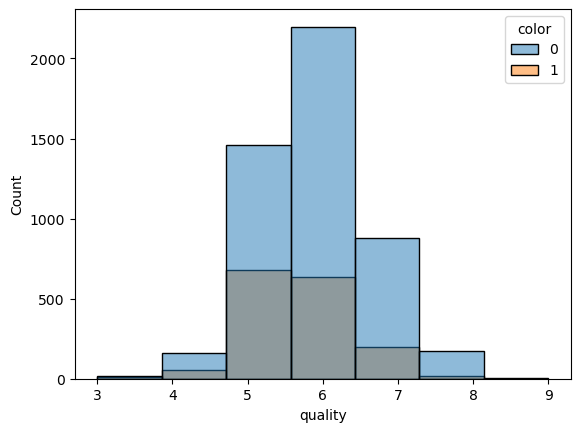
sns.pairplot(wine_df,hue='color')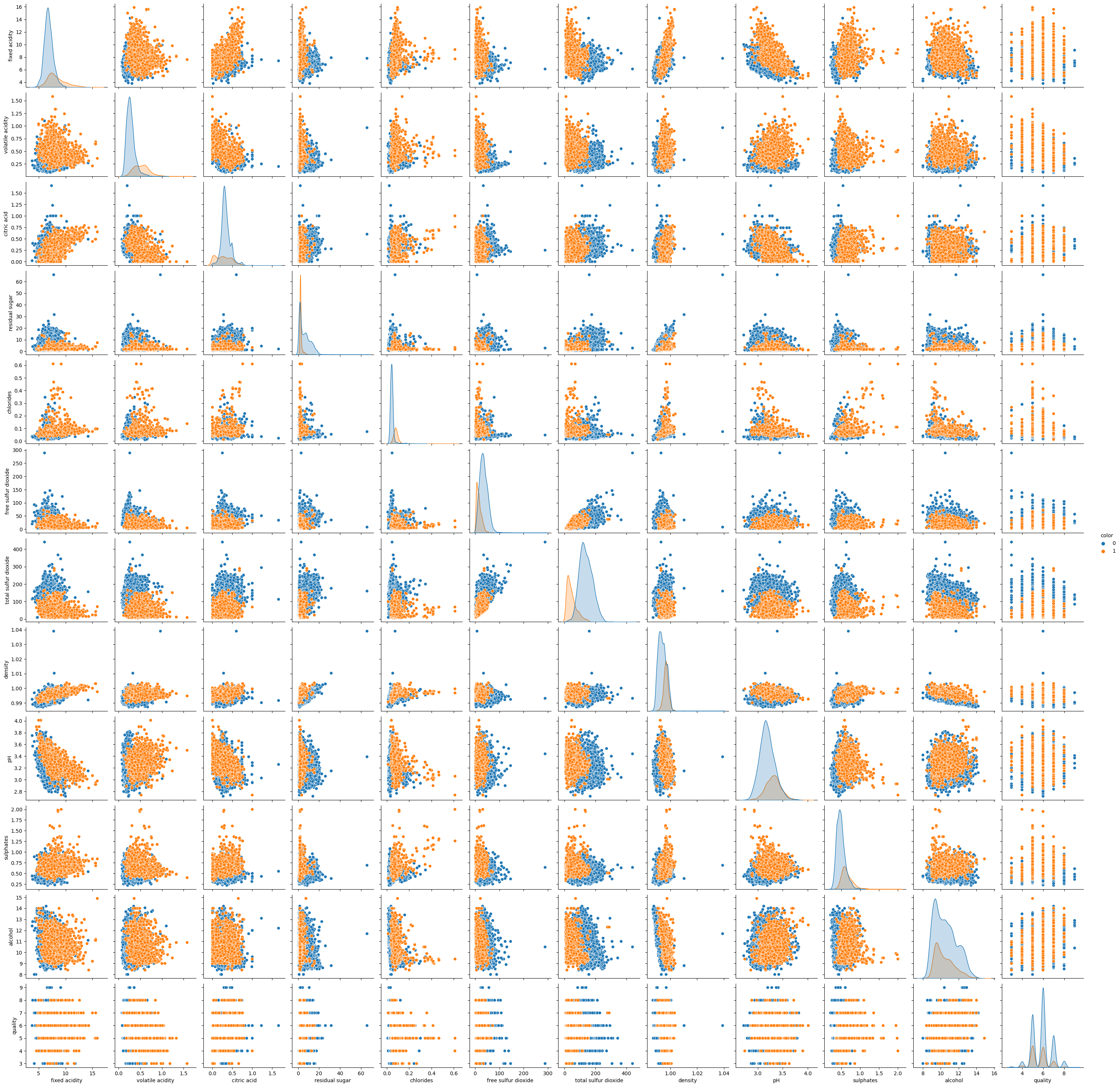
1-2. 각 feature 간의 scale이 매우 다르므로 standardscaling하기(근데 트리모델은 안해도 되긴 함)
X,y = wine_df.drop(columns=['color']),wine_df['color']from sklearn.preprocessing import StandardScaler
ss = StandardScaler()
X_scaled = ss.fit_transform(X)X_scaled = pd.DataFrame(X_scaled)
X_scaled.columns = X.columns
X_scaled| fixed acidity | volatile acidity | citric acid | residual sugar | chlorides | free sulfur dioxide | total sulfur dioxide | density | pH | sulphates | alcohol | quality | |
|---|---|---|---|---|---|---|---|---|---|---|---|---|
| 0 | -0.166089 | -0.423183 | 0.284686 | 3.206929 | -0.314975 | 0.815565 | 0.959976 | 2.102214 | -1.359049 | -0.546178 | -1.418558 | 0.207999 |
| 1 | -0.706073 | -0.240949 | 0.147046 | -0.807837 | -0.200790 | -0.931107 | 0.287618 | -0.232332 | 0.506915 | -0.277351 | -0.831615 | 0.207999 |
| 2 | 0.682458 | -0.362438 | 0.559966 | 0.306208 | -0.172244 | -0.029599 | -0.331660 | 0.134525 | 0.258120 | -0.613385 | -0.328521 | 0.207999 |
| 3 | -0.011808 | -0.666161 | 0.009406 | 0.642523 | 0.056126 | 0.928254 | 1.243074 | 0.301278 | -0.177272 | -0.882212 | -0.496219 | 0.207999 |
| 4 | -0.011808 | -0.666161 | 0.009406 | 0.642523 | 0.056126 | 0.928254 | 1.243074 | 0.301278 | -0.177272 | -0.882212 | -0.496219 | 0.207999 |
| ... | ... | ... | ... | ... | ... | ... | ... | ... | ... | ... | ... | ... |
| 6492 | -0.783214 | 1.581387 | -1.642273 | -0.723758 | 0.969605 | 0.083090 | -1.269422 | 0.067824 | 1.439897 | 0.327510 | 0.006875 | -0.937230 |
| 6493 | -1.014636 | 1.277665 | -1.504633 | -0.681719 | 0.170311 | 0.477500 | -1.145567 | 0.141195 | 1.875288 | 1.537233 | 0.593818 | 0.207999 |
| 6494 | -0.706073 | 1.034686 | -1.298173 | -0.660699 | 0.569958 | -0.085943 | -1.340197 | 0.347969 | 1.253300 | 1.470026 | 0.426120 | 0.207999 |
| 6495 | -1.014636 | 1.854738 | -1.366993 | -0.723758 | 0.541412 | 0.083090 | -1.269422 | 0.257923 | 2.186282 | 1.201199 | -0.244672 | -0.937230 |
| 6496 | -0.937495 | -0.180205 | 1.041706 | -0.387443 | 0.313042 | -0.705730 | -1.304809 | 0.264593 | 1.066704 | 0.865165 | 0.426120 | 0.207999 |
6497 rows × 12 columns
sns.pairplot(X_scaled)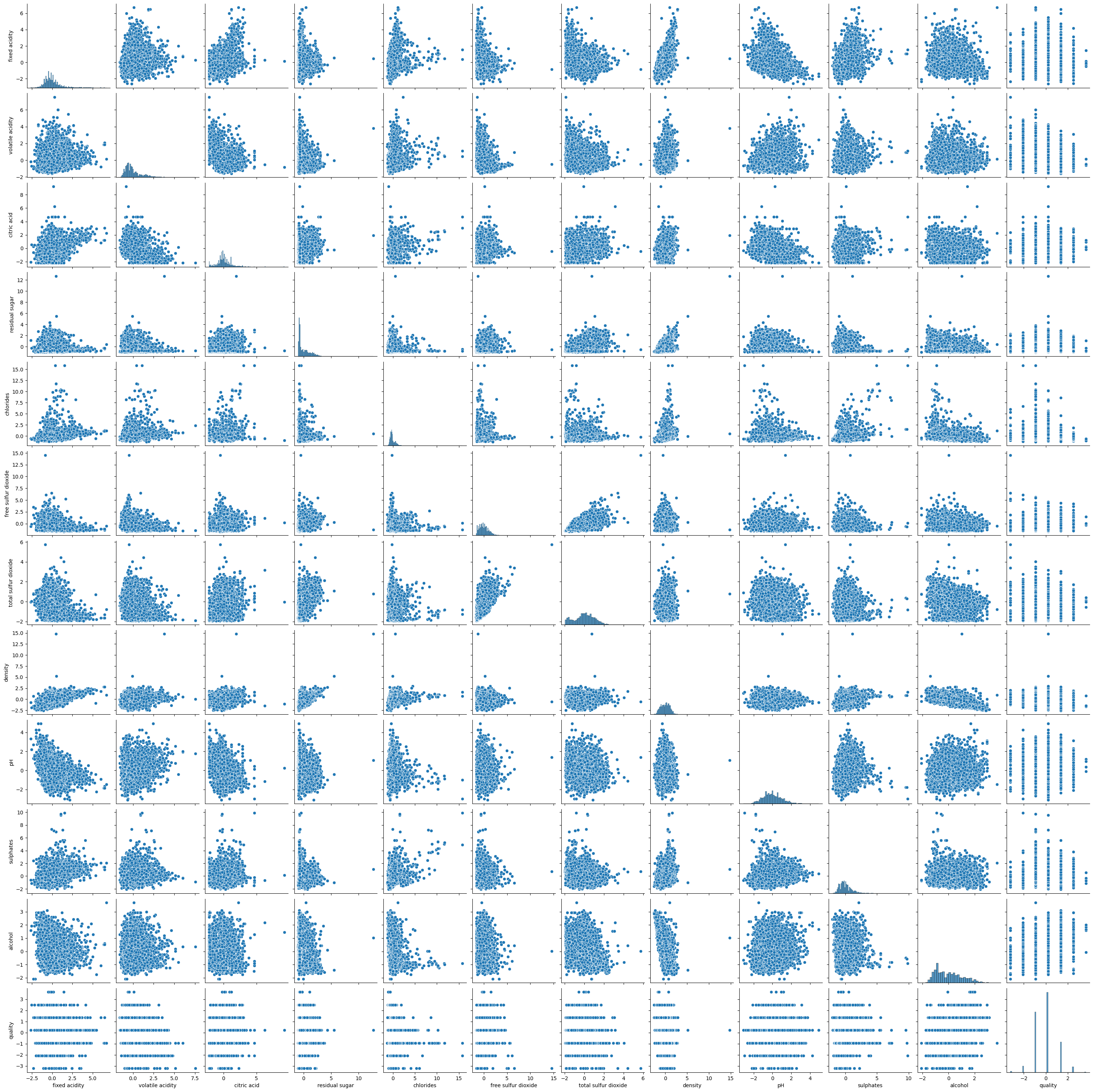
1-3. 머신러닝 모델 만들어보기
from sklearn.model_selection import train_test_split
X_train, X_test, y_train, y_test = train_test_split(X_scaled, y, test_size=0.2, random_state=42)
1-4. Accuracy Score
from sklearn.ensemble import RandomForestClassifier
rf = RandomForestClassifier(max_depth = 10, n_estimators=100,n_jobs=-1,random_state=42)
rf.fit(X_train, y_train)
rf.score(X_test, y_test)0.9961538461538462rf.predict_proba(X_test)array([[9.97449240e-01, 2.55076039e-03],
[9.88985475e-01, 1.10145251e-02],
[9.99670475e-01, 3.29524883e-04],
...,
[7.06786807e-02, 9.29321319e-01],
[2.76939341e-04, 9.99723061e-01],
[2.70729704e-04, 9.99729270e-01]])1-5. Feature_Importance
feature_imp = pd.DataFrame({'feature':X_train.columns,'importances':rf.feature_importances_})
feature_imp.sort_values(by='importances',ascending=False)| feature | importances | |
|---|---|---|
| 6 | total sulfur dioxide | 0.292221 |
| 4 | chlorides | 0.259949 |
| 1 | volatile acidity | 0.138744 |
| 5 | free sulfur dioxide | 0.055750 |
| 7 | density | 0.055543 |
| 9 | sulphates | 0.051400 |
| 3 | residual sugar | 0.050721 |
| 0 | fixed acidity | 0.046132 |
| 8 | pH | 0.022492 |
| 2 | citric acid | 0.015700 |
| 10 | alcohol | 0.009043 |
| 11 | quality | 0.002305 |
y_pred = rf.predict(X_test)1-6. Roc-Auc
from sklearn.metrics import classification_report
print(classification_report(y_test, y_pred))
precision recall f1-score support
0 0.99 1.00 1.00 986
1 1.00 0.98 0.99 314
accuracy 1.00 1300
macro avg 1.00 0.99 0.99 1300
weighted avg 1.00 1.00 1.00 1300from sklearn.metrics import RocCurveDisplay
# 예측 확률 계산 (위의 model과 X_test 사용)
y_score = rf.predict_proba(X_test)[:, 1]
# RocCurveDisplay.from_predictions 사용
RocCurveDisplay.from_predictions(y_test, y_score)
plt.show()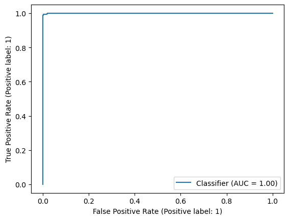
1-7. 혼동행렬(confusion matrix)
from sklearn.metrics import confusion_matrix
confusion_matrix(y_test, y_pred)
array([[986, 0],
[ 5, 309]], dtype=int64)from sklearn.metrics import ConfusionMatrixDisplay
ConfusionMatrixDisplay.from_predictions(y_test,y_pred)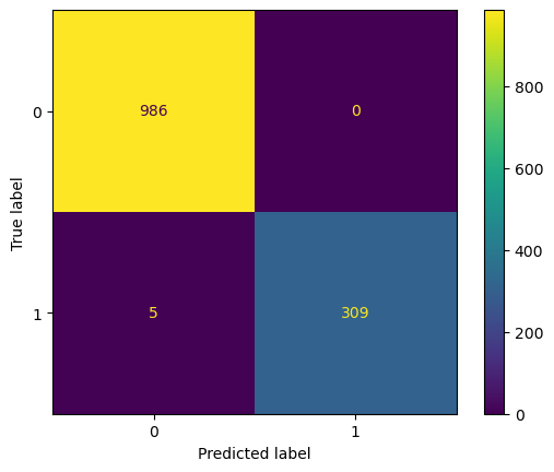
결과를 보면 실제로는 red 와인(클래스 1)인데 white 와인(클래스 0)으로 예측한 5개만 빼고 나머지는 다 맞춤
CH3-11. pipeline을 통한 모델 구성(train_test_split은 pipeline과 별도로 수행해야함)
from sklearn.pipeline import Pipeline
from sklearn.preprocessing import RobustScaler
from sklearn.model_selection import train_test_split
from sklearn.ensemble import RandomForestClassifier
from sklearn.metrics import ConfusionMatrixDisplay, RocCurveDisplay, confusion_matrix, classification_report
estimators = [('scaler',RobustScaler()),
('clf',RandomForestClassifier(max_depth = 10, n_estimators = 100, n_jobs=-1, random_state=42))]pipe = Pipeline(estimators)pipe.steps[0]('scaler', RobustScaler())pipe.steps[1]('clf', RandomForestClassifier(max_depth=10, n_jobs=-1, random_state=42))pipe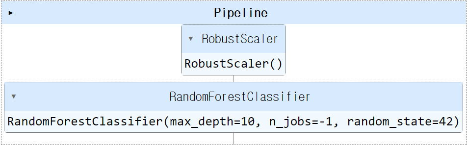
pipe.set_params(clf__max_depth=20)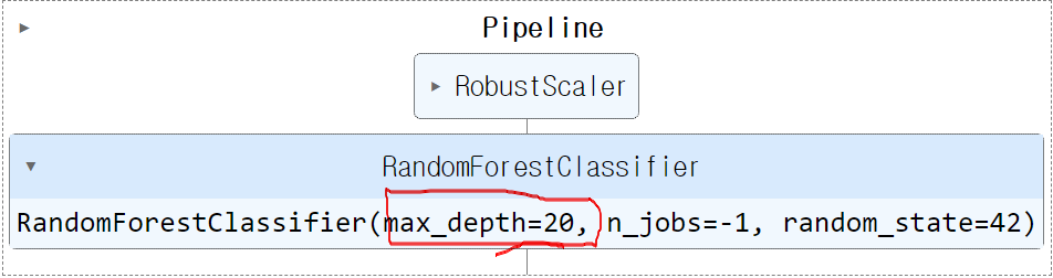
pipe.set_params(clf__random_state=2024)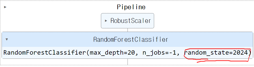
pipe['clf']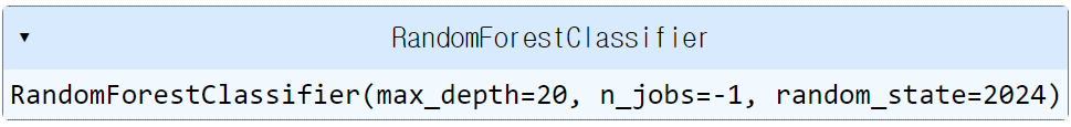
pipe['scaler']
X = wine_df.drop(columns=['color'],axis=1)
y = wine_df['color']X_train,X_test,y_train,y_test = train_test_split(X,y,test_size=0.2,random_state=2024)pipe.fit(X_train,y_train)
pipe.score(X_test,y_test)0.99461538461538461-1. test set 예측 결과 분석(classification_report, Roc-Auc Curve, Confusion Matrix)
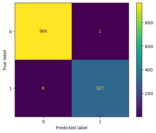
y_pred = pipe.predict(X_test)print(classification_report(y_test,y_pred)) precision recall f1-score support
0 0.99 1.00 1.00 967
1 1.00 0.98 0.99 333
accuracy 0.99 1300
macro avg 1.00 0.99 0.99 1300
weighted avg 0.99 0.99 0.99 1300RocCurveDisplay.from_predictions(y_test,y_pred)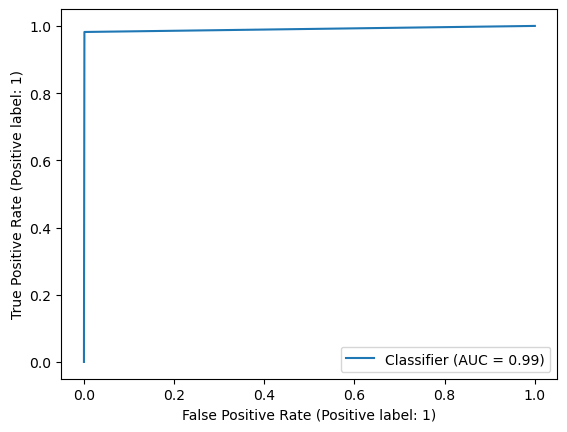
ConfusionMatrixDisplay.from_predictions(y_test,y_pred)