CH5-03: 최소자승법 OLS(Ordinary Linear Least Square)
1. 최소자승법의 수학적 원리
최소자승법(Least Squares Method)은 데이터에 대한 예측 모델의 매개변수를 추정하는 방법입니다. 이 방법은 관측된 데이터와 모델 예측 사이의 차이(잔차, residuals)의 제곱합을 최소화하여 최적의 매개변수를 찾습니다. 선형 회귀 모델에서는 보통 이 방법을 사용하여 계수를 추정합니다.
선형 회귀 모델은 다음과 같이 표현될 수 있습니다:
여기서:
- 는 관측된 종속변수 벡터입니다.
- 는 설계 행렬(design matrix)로, 각 행은 하나의 관측값에 대한 독립변수들의 값과 상수항(보통 1)을 포함합니다.
- 는 추정할 모델 매개변수(계수) 벡터입니다.
- 은 오차 항 벡터입니다.
최소자승법의 목적은 다음과 같은 비용 함수(cost function) 또는 목적 함수(objective function)를 최소화하는 를 찾는 것입니다:
를 에 대해 최소화하기 위해, 에 대한 의 미분을 0과 같게 설정합니다:
이를 재배열하면, 다음과 같은 정규 방정식(normal equations)을 얻을 수 있습니다:
이제 이 방정식을 에 대해 풀면, 최소자승 추정치를 얻을 수 있습니다:
2. 벡터, 행렬의 전치
- 전치의 교환 법칙:이 규칙은 두 행렬 A와 B의 곱셈에 대한 전치가 각각의 행렬을 전치한 후 순서를 바꿔 곱한 것과 같다는 것을 의미합니다.
- 벡터의 전치: 벡터는 1차원 행렬로 간주될 수 있으며, 행 벡터를 전치하면 열 벡터가 되고, 열 벡터를 전치하면 행 벡터가 됩니다.
이제 를 전치하면 다음과 같이 됩니다:
- 는 1×m 행렬(행 벡터),
- X는 m×n 행렬
- β는 n×1 행렬(열 벡터)입니다.
의 결과는 스칼라 값이므로, 이 스칼라 값의 전치는 그 자체와 같습니다. 그러나 표현의 목적으로 전치 연산을 적용하면, 전치 규칙에 따라 다음과 같이 표현할 수 있습니다:
이 과정에서는 다음 단계를 거칩니다:
- 의 결과는 열 벡터입니다.
- 이 열 벡터에, 즉 행 벡터를 곱하면 스칼라 값이 됩니다.
- 스칼라 값의 전치는 스칼라 값 자체와 동일합니다. 그러나 연산의 순서를 전치 규칙에 따라 바꾸면가 됩니다.
CH5-03: OLS(Ordinary Linear Least Square) 최소자승법 구현
1. 단순선형회귀를 구현해보기
import statsmodels.formula.api as smf
import pandas as pd
data = {'x':[1,2,3,4,5],'y':[1,3,4,6,5]}
df = pd.DataFrame(data)

df| x | y | |
|---|---|---|
| 0 | 1 | 1 |
| 1 | 2 | 3 |
| 2 | 3 | 4 |
| 3 | 4 | 6 |
| 4 | 5 | 5 |
## formula='y ~ x'의 의미 y=ax+b
lm_model = smf.ols(formula='y ~ x', data=df).fit()lm_model.paramsIntercept 0.5
x 1.1
dtype: float64import matplotlib.pyplot as plt
import seaborn as snsplt.figure(figsize=(10,10))
sns.lmplot(x='x', y='y',data = df)
plt.xlim([0,5])
plt.show()
<Figure size 1000x1000 with 0 Axes>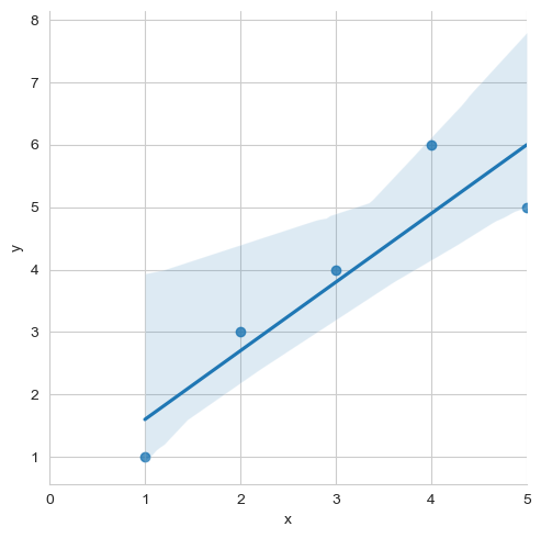
1-2. 잔차(Residual)은 평균이 0이고 정규분포를 따라야함
- 잔차 = 실제값-예측값
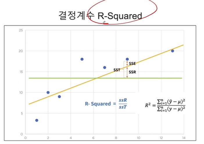
2. numpy를 통해 직접 결정계수 계산해보기
결정계수(R-squared)는 회귀제곱합(SSR)/SST:
즉, 오차가 회귀로 에측되는 정도를 측정하므로 높을 수록 좋음
import numpy as np
mu = np.mean(df['y'])
y = df['y']
y_hat = lm_model.predict()
np.sum((y_hat-mu)**2)/np.sum((y-mu)**2)0.8175675675675671lm_model.rsquared0.8175675675675677CH5-04 통계적 회귀
import pandas as pd
import numpy as np
import matplotlib.pyplot as plt
import seaborn as snsurl = 'https://raw.githubusercontent.com/PinkWink/ML_tutorial/master/dataset/ecommerce.csv'
df = pd.read_csv(url, sep = ',', encoding='utf-8')df| Address | Avatar | Avg. Session Length | Time on App | Time on Website | Length of Membership | Yearly Amount Spent | ||
|---|---|---|---|---|---|---|---|---|
| 0 | mstephenson@fernandez.com | 835 Frank Tunnel\nWrightmouth, MI 82180-9605 | Violet | 34.497268 | 12.655651 | 39.577668 | 4.082621 | 587.951054 |
| 1 | hduke@hotmail.com | 4547 Archer Common\nDiazchester, CA 06566-8576 | DarkGreen | 31.926272 | 11.109461 | 37.268959 | 2.664034 | 392.204933 |
| 2 | pallen@yahoo.com | 24645 Valerie Unions Suite 582\nCobbborough, D... | Bisque | 33.000915 | 11.330278 | 37.110597 | 4.104543 | 487.547505 |
| 3 | riverarebecca@gmail.com | 1414 David Throughway\nPort Jason, OH 22070-1220 | SaddleBrown | 34.305557 | 13.717514 | 36.721283 | 3.120179 | 581.852344 |
| 4 | mstephens@davidson-herman.com | 14023 Rodriguez Passage\nPort Jacobville, PR 3... | MediumAquaMarine | 33.330673 | 12.795189 | 37.536653 | 4.446308 | 599.406092 |
| ... | ... | ... | ... | ... | ... | ... | ... | ... |
| 495 | lewisjessica@craig-evans.com | 4483 Jones Motorway Suite 872\nLake Jamiefurt,... | Tan | 33.237660 | 13.566160 | 36.417985 | 3.746573 | 573.847438 |
| 496 | katrina56@gmail.com | 172 Owen Divide Suite 497\nWest Richard, CA 19320 | PaleVioletRed | 34.702529 | 11.695736 | 37.190268 | 3.576526 | 529.049004 |
| 497 | dale88@hotmail.com | 0787 Andrews Ranch Apt. 633\nSouth Chadburgh, ... | Cornsilk | 32.646777 | 11.499409 | 38.332576 | 4.958264 | 551.620145 |
| 498 | cwilson@hotmail.com | 680 Jennifer Lodge Apt. 808\nBrendachester, TX... | Teal | 33.322501 | 12.391423 | 36.840086 | 2.336485 | 456.469510 |
| 499 | hannahwilson@davidson.com | 49791 Rachel Heights Apt. 898\nEast Drewboroug... | DarkMagenta | 33.715981 | 12.418808 | 35.771016 | 2.735160 | 497.778642 |
500 rows × 8 columns
칼럼명세
- Avg. Session Length: 한 번 접속시 평균 사용시간
- Time on App: 폰 앱으로 접속시 유지시간(분)
- Time on Website: 웹사이트로 접속시 유지시간(분)
- Length of Membership: 회원 자격 유지 기간(년)
- Yearly Amount Spent: 타겟값임(연간 소비액)
df.info()<class 'pandas.core.frame.DataFrame'>
RangeIndex: 500 entries, 0 to 499
Data columns (total 8 columns):
# Column Non-Null Count Dtype
--- ------ -------------- -----
0 Email 500 non-null object
1 Address 500 non-null object
2 Avatar 500 non-null object
3 Avg. Session Length 500 non-null float64
4 Time on App 500 non-null float64
5 Time on Website 500 non-null float64
6 Length of Membership 500 non-null float64
7 Yearly Amount Spent 500 non-null float64
dtypes: float64(5), object(3)
memory usage: 31.4+ KB1. 불필요한 칼럼 삭제
df = df.drop(columns=['Avatar','Address','Email'], axis = 1)
df| Avg. Session Length | Time on App | Time on Website | Length of Membership | Yearly Amount Spent | |
|---|---|---|---|---|---|
| 0 | 34.497268 | 12.655651 | 39.577668 | 4.082621 | 587.951054 |
| 1 | 31.926272 | 11.109461 | 37.268959 | 2.664034 | 392.204933 |
| 2 | 33.000915 | 11.330278 | 37.110597 | 4.104543 | 487.547505 |
| 3 | 34.305557 | 13.717514 | 36.721283 | 3.120179 | 581.852344 |
| 4 | 33.330673 | 12.795189 | 37.536653 | 4.446308 | 599.406092 |
| ... | ... | ... | ... | ... | ... |
| 495 | 33.237660 | 13.566160 | 36.417985 | 3.746573 | 573.847438 |
| 496 | 34.702529 | 11.695736 | 37.190268 | 3.576526 | 529.049004 |
| 497 | 32.646777 | 11.499409 | 38.332576 | 4.958264 | 551.620145 |
| 498 | 33.322501 | 12.391423 | 36.840086 | 2.336485 | 456.469510 |
| 499 | 33.715981 | 12.418808 | 35.771016 | 2.735160 | 497.778642 |
500 rows × 5 columns
df.info()<class 'pandas.core.frame.DataFrame'>
RangeIndex: 500 entries, 0 to 499
Data columns (total 5 columns):
# Column Non-Null Count Dtype
--- ------ -------------- -----
0 Avg. Session Length 500 non-null float64
1 Time on App 500 non-null float64
2 Time on Website 500 non-null float64
3 Length of Membership 500 non-null float64
4 Yearly Amount Spent 500 non-null float64
dtypes: float64(5)
memory usage: 19.7 KB3. feature와 target의 박스플랏
plt.figure(figsize=(10,10))
sns.boxplot(data=df.iloc[:,:4])<Axes: >
plt.figure(figsize=(10,10))
sns.boxplot(data=df.iloc[:,4]).set_xlabel('Yearly Amount Spent')
Text(0.5, 0, 'Yearly Amount Spent')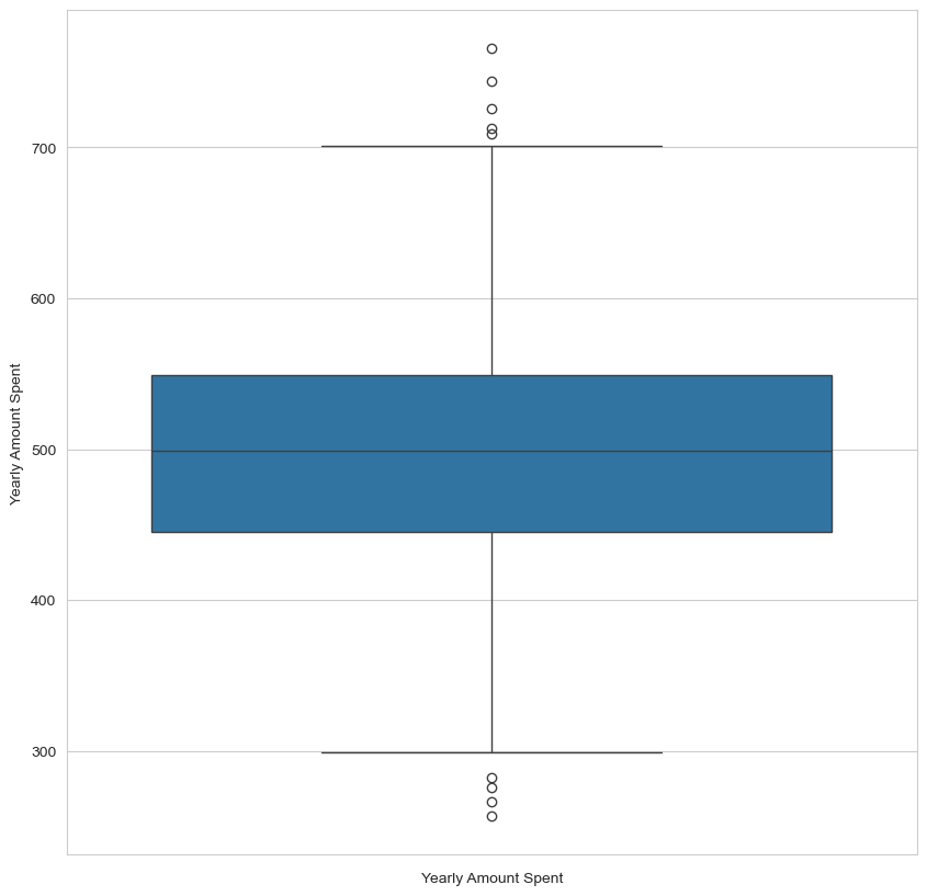
plt.figure(figsize=(12,12))
sns.pairplot(df)<seaborn.axisgrid.PairGrid at 0x1fbc24e4350>
<Figure size 1200x1200 with 0 Axes>
4. Length of Membership과 Yearly Amount Spent의 상관관계가 가장 커보임
sns.lmplot(data=df,x='Length of Membership', y='Yearly Amount Spent')<seaborn.axisgrid.FacetGrid at 0x1fbc3046b10>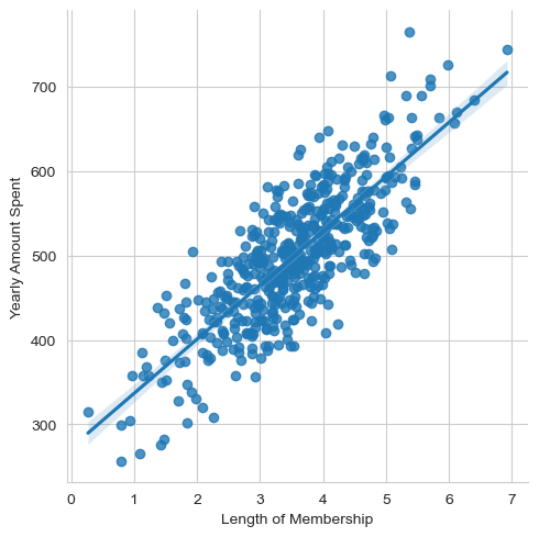
5. Length of Membership만 활용하여 단순선형회귀 구현하기
import statsmodels.api as sm
import matplotlib.pyplot as plt
X = df['Length of Membership']
y = df['Yearly Amount Spent']
lm = sm.OLS(y,X).fit()
lm.summary()| Dep. Variable: | Yearly Amount Spent | R-squared (uncentered): | 0.970 |
|---|---|---|---|
| Model: | OLS | Adj. R-squared (uncentered): | 0.970 |
| Method: | Least Squares | F-statistic: | 1.617e+04 |
| Date: | Sat, 17 Feb 2024 | Prob (F-statistic): | 0.00 |
| Time: | 02:21:09 | Log-Likelihood: | -2945.2 |
| No. Observations: | 500 | AIC: | 5892. |
| Df Residuals: | 499 | BIC: | 5897. |
| Df Model: | 1 | ||
| Covariance Type: | nonrobust |
| coef | std err | t | P>|t| | [0.025 | 0.975] | |
|---|---|---|---|---|---|---|
| Length of Membership | 135.6117 | 1.067 | 127.145 | 0.000 | 133.516 | 137.707 |
| Omnibus: | 1.408 | Durbin-Watson: | 1.975 |
|---|---|---|---|
| Prob(Omnibus): | 0.494 | Jarque-Bera (JB): | 1.472 |
| Skew: | 0.125 | Prob(JB): | 0.479 |
| Kurtosis: | 2.909 | Cond. No. | 1.00 |
Notes:
[1] R² is computed without centering (uncentered) since the model does not contain a constant.
[2] Standard Errors assume that the covariance matrix of the errors is correctly specified.
pred = lm.predict(X)
sns.scatterplot(x=X,y=y)
plt.plot(X,pred, ls = 'dashed', color = 'red')
plt.show()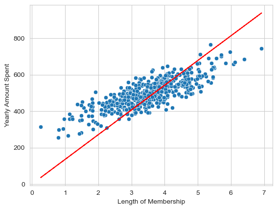
6. 상수항을 추가하기
X = np.c_[X,len(X)*[1]]
X[:5]
array([[4.08262063, 1. ],
[2.66403418, 1. ],
[4.1045432 , 1. ],
[3.12017878, 1. ],
[4.44630832, 1. ]])lm = sm.OLS(y,X).fit()
lm.summary()| Dep. Variable: | Yearly Amount Spent | R-squared: | 0.655 |
|---|---|---|---|
| Model: | OLS | Adj. R-squared: | 0.654 |
| Method: | Least Squares | F-statistic: | 943.9 |
| Date: | Sat, 17 Feb 2024 | Prob (F-statistic): | 4.81e-117 |
| Time: | 02:21:09 | Log-Likelihood: | -2629.9 |
| No. Observations: | 500 | AIC: | 5264. |
| Df Residuals: | 498 | BIC: | 5272. |
| Df Model: | 1 | ||
| Covariance Type: | nonrobust |
| coef | std err | t | P>|t| | [0.025 | 0.975] | |
|---|---|---|---|---|---|---|
| x1 | 64.2187 | 2.090 | 30.723 | 0.000 | 60.112 | 68.326 |
| const | 272.3998 | 7.675 | 35.492 | 0.000 | 257.320 | 287.479 |
| Omnibus: | 1.092 | Durbin-Watson: | 2.065 |
|---|---|---|---|
| Prob(Omnibus): | 0.579 | Jarque-Bera (JB): | 1.122 |
| Skew: | 0.037 | Prob(JB): | 0.571 |
| Kurtosis: | 2.780 | Cond. No. | 14.4 |
Notes:
[1] Standard Errors assume that the covariance matrix of the errors is correctly specified.
y_pred = lm.predict(X)
sns.scatterplot(x=X[:,0], y=y)
plt.plot(X[:,0],y_pred,color='red')
plt.ylabel('Yearly Amount Spent')
plt.show()
7. 사이킷런을 통해 선형회귀 구현
X = df.drop(columns = 'Yearly Amount Spent', axis = 1)
y = df['Yearly Amount Spent']
from sklearn.model_selection import train_test_split
X_train,X_test,y_train,y_test = train_test_split(X,y, test_size = 0.2, random_state = 2024)from sklearn.linear_model import LinearRegression
lr = LinearRegression()
lr.fit(X_train, y_train)
lr.score(X_test, y_test)0.9822087908914663X_test| Avg. Session Length | Time on App | Time on Website | Length of Membership | |
|---|---|---|---|---|
| 243 | 32.454553 | 11.822983 | 36.946126 | 3.656984 |
| 306 | 31.912076 | 11.792972 | 36.257819 | 2.395168 |
| 56 | 32.688229 | 13.761533 | 39.252931 | 2.995761 |
| 113 | 32.653181 | 11.602532 | 37.309689 | 2.789462 |
| 236 | 32.693240 | 12.600750 | 37.370118 | 3.467014 |
| ... | ... | ... | ... | ... |
| 365 | 32.030550 | 12.644202 | 38.001827 | 5.038107 |
| 418 | 31.673916 | 12.329147 | 37.074371 | 3.982462 |
| 33 | 32.728360 | 13.104507 | 38.878041 | 2.820097 |
| 103 | 33.437830 | 12.595420 | 36.262032 | 2.969640 |
| 486 | 33.452295 | 12.005916 | 36.534096 | 4.712234 |
100 rows × 4 columns
회귀계수와 절편
lr.coef_array([25.71840741, 38.77908883, 0.164811 , 61.9778141 ])lr.intercept_-1043.4700878021783CH5-05 비용함수(선형회귀의 경우는 MSE)의 최소값 찾기
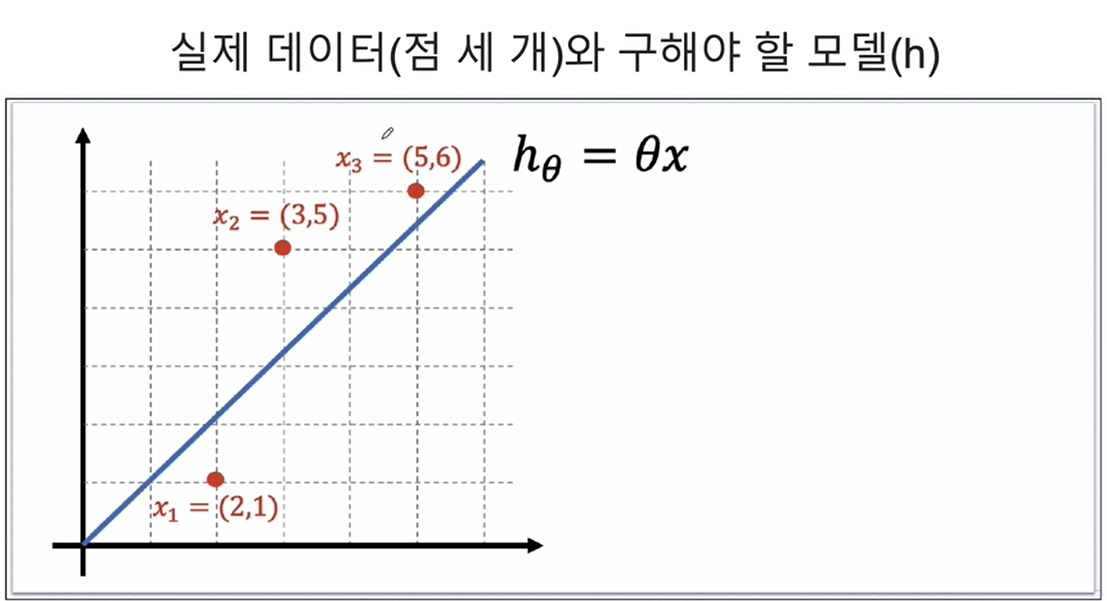
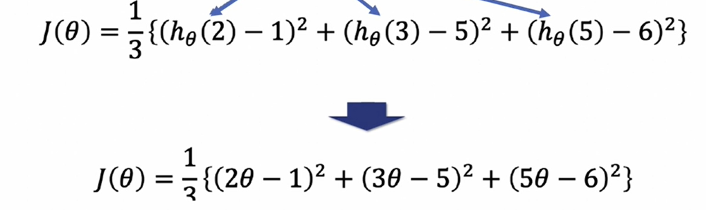
import sympy as sym1. 위 표의 실제값, 예측값에 대해 Cost Function(MSE) 구하기
''
- 즉, '$38x^2 - 94x + 62 $' 을 넘파이로 표현한 식이 밑의 식임
- np.poly1d([])에서 리스트 안의 값은 가장 마지막 인덱스가 상수항이며 앞으로 갈수록 차수가 높아짐(1개 변수의 다항식 표현)
np.poly1d([2,-1])**2 + np.poly1d([3, -5])**2 + np.poly1d([5,-6])**2poly1d([ 38, -94, 62])1. sympy를 통해 미분하기
theta = sym.Symbol('theta')
diff = sym.diff(38*theta**2 - 94*theta + 62, theta)
diff
f = np.poly1d([2,-1])**2 + np.poly1d([3, -5])**2 + np.poly1d([5,-6])**2theta2 = np.linspace(-10, 10, 100)
di = f.deriv()
cost_diff = di(theta2)2. 즉, cost function인 ''는 미분 함수인 ''와 y=0이 교차하는 x값에서 최소값을 가짐
plt.plot(theta2, cost_diff, color='r',ls='--', label = r'$76\theta - 94$')
plt.title(r'$76\theta - 94$',fontsize=20)
plt.legend()
plt.axhline(y=0)
plt.xlabel(r'$\theta$', fontsize = 20)
plt.ylabel(r'$f(\theta)$', fontsize=20)
plt.show()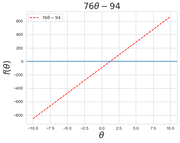
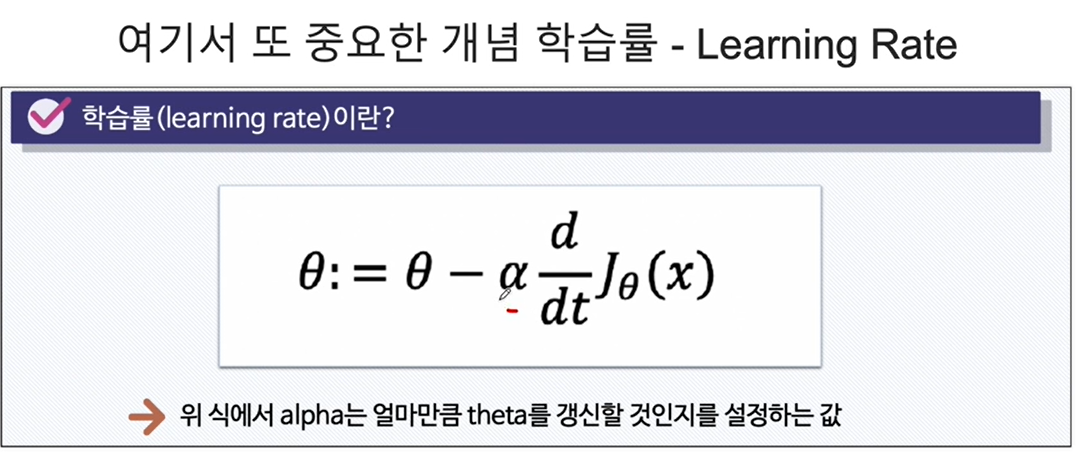
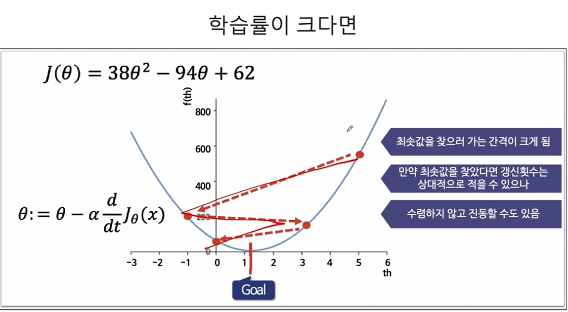
CH5-06 Gradient Descent(경사하강법)
- 처음에는 임의의 랜덤한 theta를 선택함


CH5-07: 보스턴 주택 가격 회귀 분석(1)

url ='https://raw.githubusercontent.com/PinkWink/ML_tutorial/master/dataset/boston.csv'
boston = pd.read_csv(url)
boston.info()<class 'pandas.core.frame.DataFrame'>
RangeIndex: 506 entries, 0 to 505
Data columns (total 14 columns):
# Column Non-Null Count Dtype
--- ------ -------------- -----
0 CRIM 506 non-null float64
1 ZN 506 non-null float64
2 INDUS 506 non-null float64
3 CHAS 506 non-null int64
4 NOX 506 non-null float64
5 RM 506 non-null float64
6 AGE 506 non-null float64
7 DIS 506 non-null float64
8 RAD 506 non-null int64
9 TAX 506 non-null float64
10 PTRATIO 506 non-null float64
11 B 506 non-null float64
12 LSTAT 506 non-null float64
13 MEDV 506 non-null float64
dtypes: float64(12), int64(2)
memory usage: 55.5 KBboston.describe()| CRIM | ZN | INDUS | CHAS | NOX | RM | AGE | DIS | RAD | TAX | PTRATIO | B | LSTAT | MEDV | |
|---|---|---|---|---|---|---|---|---|---|---|---|---|---|---|
| count | 506.000000 | 506.000000 | 506.000000 | 506.000000 | 506.000000 | 506.000000 | 506.000000 | 506.000000 | 506.000000 | 506.000000 | 506.000000 | 506.000000 | 506.000000 | 506.000000 |
| mean | 3.613524 | 11.363636 | 11.136779 | 0.069170 | 0.554695 | 6.284634 | 68.574901 | 3.795043 | 9.549407 | 408.237154 | 18.455534 | 356.674032 | 12.653063 | 22.532806 |
| std | 8.601545 | 23.322453 | 6.860353 | 0.253994 | 0.115878 | 0.702617 | 28.148861 | 2.105710 | 8.707259 | 168.537116 | 2.164946 | 91.294864 | 7.141062 | 9.197104 |
| min | 0.006320 | 0.000000 | 0.460000 | 0.000000 | 0.385000 | 3.561000 | 2.900000 | 1.129600 | 1.000000 | 187.000000 | 12.600000 | 0.320000 | 1.730000 | 5.000000 |
| 25% | 0.082045 | 0.000000 | 5.190000 | 0.000000 | 0.449000 | 5.885500 | 45.025000 | 2.100175 | 4.000000 | 279.000000 | 17.400000 | 375.377500 | 6.950000 | 17.025000 |
| 50% | 0.256510 | 0.000000 | 9.690000 | 0.000000 | 0.538000 | 6.208500 | 77.500000 | 3.207450 | 5.000000 | 330.000000 | 19.050000 | 391.440000 | 11.360000 | 21.200000 |
| 75% | 3.677083 | 12.500000 | 18.100000 | 0.000000 | 0.624000 | 6.623500 | 94.075000 | 5.188425 | 24.000000 | 666.000000 | 20.200000 | 396.225000 | 16.955000 | 25.000000 |
| max | 88.976200 | 100.000000 | 27.740000 | 1.000000 | 0.871000 | 8.780000 | 100.000000 | 12.126500 | 24.000000 | 711.000000 | 22.000000 | 396.900000 | 37.970000 | 50.000000 |
boston.head()| CRIM | ZN | INDUS | CHAS | NOX | RM | AGE | DIS | RAD | TAX | PTRATIO | B | LSTAT | MEDV | |
|---|---|---|---|---|---|---|---|---|---|---|---|---|---|---|
| 0 | 0.00632 | 18.0 | 2.31 | 0 | 0.538 | 6.575 | 65.2 | 4.0900 | 1 | 296.0 | 15.3 | 396.90 | 4.98 | 24.0 |
| 1 | 0.02731 | 0.0 | 7.07 | 0 | 0.469 | 6.421 | 78.9 | 4.9671 | 2 | 242.0 | 17.8 | 396.90 | 9.14 | 21.6 |
| 2 | 0.02729 | 0.0 | 7.07 | 0 | 0.469 | 7.185 | 61.1 | 4.9671 | 2 | 242.0 | 17.8 | 392.83 | 4.03 | 34.7 |
| 3 | 0.03237 | 0.0 | 2.18 | 0 | 0.458 | 6.998 | 45.8 | 6.0622 | 3 | 222.0 | 18.7 | 394.63 | 2.94 | 33.4 |
| 4 | 0.06905 | 0.0 | 2.18 | 0 | 0.458 | 7.147 | 54.2 | 6.0622 | 3 | 222.0 | 18.7 | 396.90 | 5.33 | 36.2 |
import plotly.express as px1. PRICE(MEDV)의 히스토그램
fig = px.histogram(boston, 'MEDV')
fig.show()
2. 상관계수 히트맵
corr_matrix = boston.corr(method = 'pearson')
corr_matrix| CRIM | ZN | INDUS | CHAS | NOX | RM | AGE | DIS | RAD | TAX | PTRATIO | B | LSTAT | MEDV | |
|---|---|---|---|---|---|---|---|---|---|---|---|---|---|---|
| CRIM | 1.000000 | -0.200469 | 0.406583 | -0.055892 | 0.420972 | -0.219247 | 0.352734 | -0.379670 | 0.625505 | 0.582764 | 0.289946 | -0.385064 | 0.455621 | -0.388305 |
| ZN | -0.200469 | 1.000000 | -0.533828 | -0.042697 | -0.516604 | 0.311991 | -0.569537 | 0.664408 | -0.311948 | -0.314563 | -0.391679 | 0.175520 | -0.412995 | 0.360445 |
| INDUS | 0.406583 | -0.533828 | 1.000000 | 0.062938 | 0.763651 | -0.391676 | 0.644779 | -0.708027 | 0.595129 | 0.720760 | 0.383248 | -0.356977 | 0.603800 | -0.483725 |
| CHAS | -0.055892 | -0.042697 | 0.062938 | 1.000000 | 0.091203 | 0.091251 | 0.086518 | -0.099176 | -0.007368 | -0.035587 | -0.121515 | 0.048788 | -0.053929 | 0.175260 |
| NOX | 0.420972 | -0.516604 | 0.763651 | 0.091203 | 1.000000 | -0.302188 | 0.731470 | -0.769230 | 0.611441 | 0.668023 | 0.188933 | -0.380051 | 0.590879 | -0.427321 |
| RM | -0.219247 | 0.311991 | -0.391676 | 0.091251 | -0.302188 | 1.000000 | -0.240265 | 0.205246 | -0.209847 | -0.292048 | -0.355501 | 0.128069 | -0.613808 | 0.695360 |
| AGE | 0.352734 | -0.569537 | 0.644779 | 0.086518 | 0.731470 | -0.240265 | 1.000000 | -0.747881 | 0.456022 | 0.506456 | 0.261515 | -0.273534 | 0.602339 | -0.376955 |
| DIS | -0.379670 | 0.664408 | -0.708027 | -0.099176 | -0.769230 | 0.205246 | -0.747881 | 1.000000 | -0.494588 | -0.534432 | -0.232471 | 0.291512 | -0.496996 | 0.249929 |
| RAD | 0.625505 | -0.311948 | 0.595129 | -0.007368 | 0.611441 | -0.209847 | 0.456022 | -0.494588 | 1.000000 | 0.910228 | 0.464741 | -0.444413 | 0.488676 | -0.381626 |
| TAX | 0.582764 | -0.314563 | 0.720760 | -0.035587 | 0.668023 | -0.292048 | 0.506456 | -0.534432 | 0.910228 | 1.000000 | 0.460853 | -0.441808 | 0.543993 | -0.468536 |
| PTRATIO | 0.289946 | -0.391679 | 0.383248 | -0.121515 | 0.188933 | -0.355501 | 0.261515 | -0.232471 | 0.464741 | 0.460853 | 1.000000 | -0.177383 | 0.374044 | -0.507787 |
| B | -0.385064 | 0.175520 | -0.356977 | 0.048788 | -0.380051 | 0.128069 | -0.273534 | 0.291512 | -0.444413 | -0.441808 | -0.177383 | 1.000000 | -0.366087 | 0.333461 |
| LSTAT | 0.455621 | -0.412995 | 0.603800 | -0.053929 | 0.590879 | -0.613808 | 0.602339 | -0.496996 | 0.488676 | 0.543993 | 0.374044 | -0.366087 | 1.000000 | -0.737663 |
| MEDV | -0.388305 | 0.360445 | -0.483725 | 0.175260 | -0.427321 | 0.695360 | -0.376955 | 0.249929 | -0.381626 | -0.468536 | -0.507787 | 0.333461 | -0.737663 | 1.000000 |
plt.figure(figsize=(13,13))
sns.heatmap(corr_matrix, annot=True)
plt.show()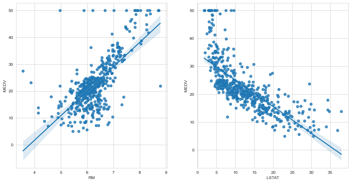
2. MEDV(PRICE)와 가장 상관관계가 강한 피처는 RM과 LSTAT이므로 RM과 LSTAT을 더 분석해보기
sns.set_style('whitegrid')
fig, axes = plt.subplots(1,2,figsize=(14,7))
sns.regplot(data=boston, x='RM', y='MEDV',ax = axes[0])
sns.regplot(data=boston, x='LSTAT', y='MEDV',ax=axes[1])
plt.show()
X, y = boston.drop('MEDV',axis=1), np.array(boston['MEDV'])from sklearn.model_selection import train_test_split
X_train,X_test,y_train,y_test = train_test_split(X,y,test_size=0.2,random_state=2024)from sklearn.linear_model import LinearRegression
lr = LinearRegression()
lr.fit(X_train,y_train)lr.score(X_test,y_test)0.7913054941937426from sklearn.metrics import mean_squared_error
y_pred_test = lr.predict(X_test)
rmse = np.sqrt(mean_squared_error(y_test, y_pred_test))
rmse4.486505110455414q1 = boston['MEDV'].quantile(0.25)
q2 = boston['MEDV'].quantile(0.5)
q3 = boston['MEDV'].quantile(0.75)
iqr = q3-q1
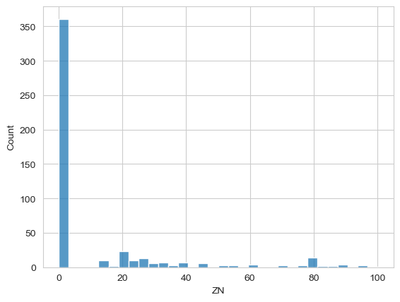
ceiling = q3 + iqr * 3ceiling48.925000000000004피처엔지니어링 및 이상치 탐지 제거
boston_new = boston.copy()sns.histplot(boston_new, x='ZN')<Axes: xlabel='ZN', ylabel='Count'>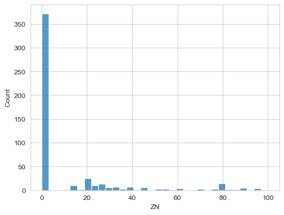
boston_new| CRIM | ZN | INDUS | CHAS | NOX | RM | AGE | DIS | RAD | TAX | PTRATIO | B | LSTAT | MEDV | |
|---|---|---|---|---|---|---|---|---|---|---|---|---|---|---|
| 0 | 0.00632 | 18.0 | 2.31 | 0 | 0.538 | 6.575 | 65.2 | 4.0900 | 1 | 296.0 | 15.3 | 396.90 | 4.98 | 24.0 |
| 1 | 0.02731 | 0.0 | 7.07 | 0 | 0.469 | 6.421 | 78.9 | 4.9671 | 2 | 242.0 | 17.8 | 396.90 | 9.14 | 21.6 |
| 2 | 0.02729 | 0.0 | 7.07 | 0 | 0.469 | 7.185 | 61.1 | 4.9671 | 2 | 242.0 | 17.8 | 392.83 | 4.03 | 34.7 |
| 3 | 0.03237 | 0.0 | 2.18 | 0 | 0.458 | 6.998 | 45.8 | 6.0622 | 3 | 222.0 | 18.7 | 394.63 | 2.94 | 33.4 |
| 4 | 0.06905 | 0.0 | 2.18 | 0 | 0.458 | 7.147 | 54.2 | 6.0622 | 3 | 222.0 | 18.7 | 396.90 | 5.33 | 36.2 |
| ... | ... | ... | ... | ... | ... | ... | ... | ... | ... | ... | ... | ... | ... | ... |
| 501 | 0.06263 | 0.0 | 11.93 | 0 | 0.573 | 6.593 | 69.1 | 2.4786 | 1 | 273.0 | 21.0 | 391.99 | 9.67 | 22.4 |
| 502 | 0.04527 | 0.0 | 11.93 | 0 | 0.573 | 6.120 | 76.7 | 2.2875 | 1 | 273.0 | 21.0 | 396.90 | 9.08 | 20.6 |
| 503 | 0.06076 | 0.0 | 11.93 | 0 | 0.573 | 6.976 | 91.0 | 2.1675 | 1 | 273.0 | 21.0 | 396.90 | 5.64 | 23.9 |
| 504 | 0.10959 | 0.0 | 11.93 | 0 | 0.573 | 6.794 | 89.3 | 2.3889 | 1 | 273.0 | 21.0 | 393.45 | 6.48 | 22.0 |
| 505 | 0.04741 | 0.0 | 11.93 | 0 | 0.573 | 6.030 | 80.8 | 2.5050 | 1 | 273.0 | 21.0 | 396.90 | 7.88 | 11.9 |
506 rows × 14 columns
sns.regplot(boston_new, x='PTRATIO', y='MEDV')<Axes: xlabel='PTRATIO', ylabel='MEDV'>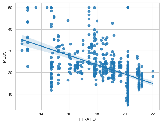
sns.regplot(boston_new, x='AGE', y='MEDV')<Axes: xlabel='AGE', ylabel='MEDV'>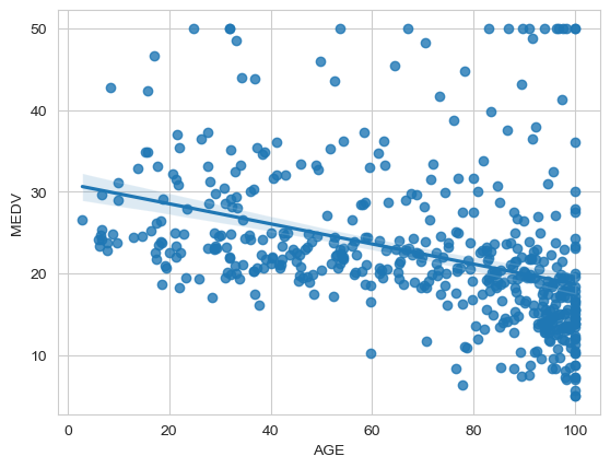
sns.pairplot(boston_new)<seaborn.axisgrid.PairGrid at 0x1b19b263190>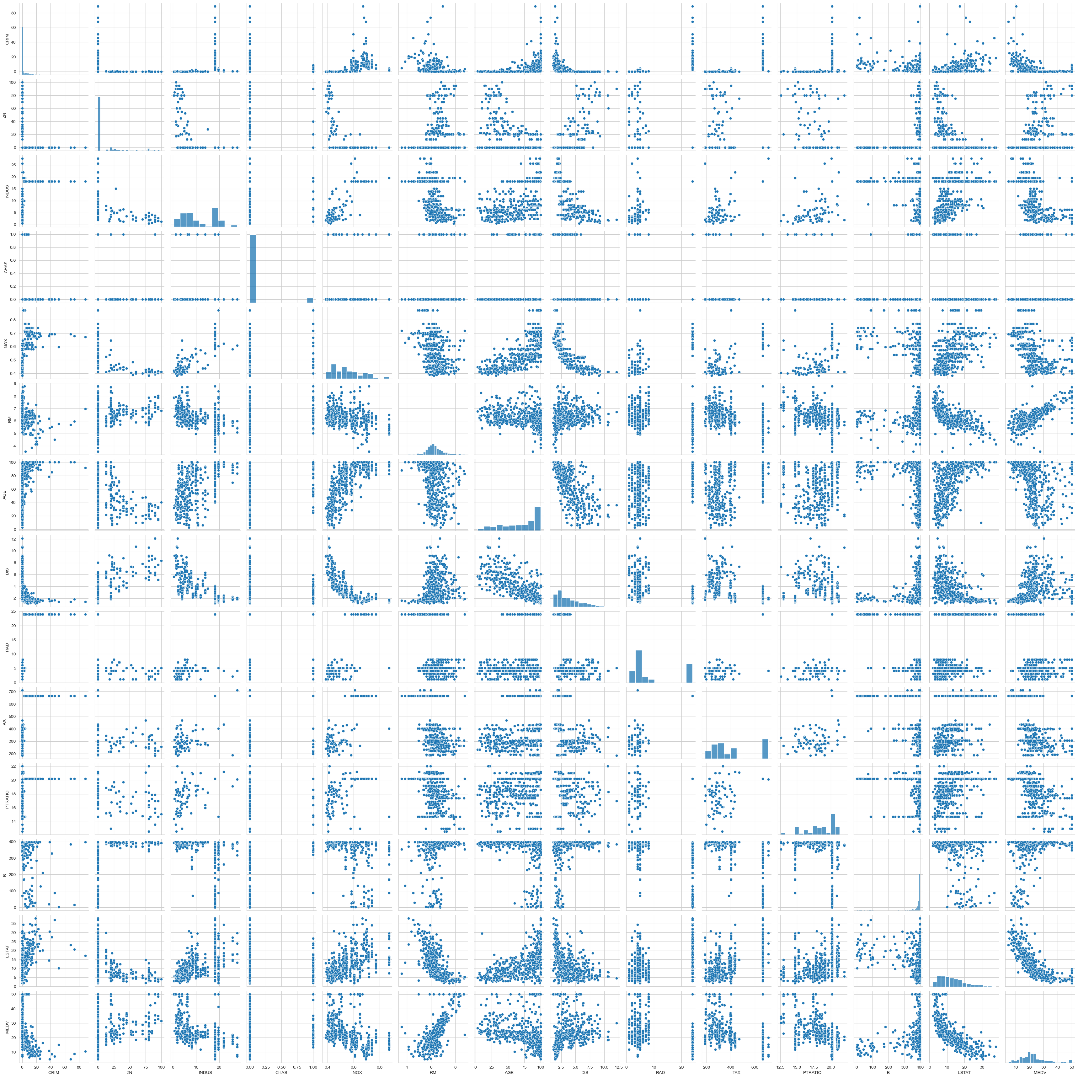
boston_new.loc[:,'INDAGENOX'] = boston_new.loc[:,'INDUS'] * boston_new.loc[:,'NOX'] * boston_new.loc[:,'AGE']
boston_new.loc[:,'RMDIS'] = boston_new.loc[:,'RM'] ** 2 * boston_new.loc[:,'DIS']
boston_new.loc[:,'LSTATAGE'] = boston_new.loc[:,'LSTAT'] ** 2 * boston_new.loc[:,'AGE']
boston_new.loc[:,'RMLSTAT'] = boston_new.loc[:,'RM'] ** 2 * boston_new.loc[:,'LSTAT']
boston_new.loc[:,'DISLSTAT'] = boston_new.loc[:,'DIS'] * boston_new.loc[:,'LSTAT']
모델 정규화 및 훈련세트분리 및 이상치 제거(이상치 제거시에는 Train set에만 적용시켰다)
train, test = train_test_split(boston_new, test_size = 0.2, random_state=2024)# 이상치 제거 함수 정의
def remove_outliers(df, column):
Q1 = df[column].quantile(0.25)
Q3 = df[column].quantile(0.75)
IQR = Q3 - Q1
lower_bound = Q1 - 1.5 * IQR
upper_bound = Q3 + 1.5 * IQR
# 이상치가 아닌 값만 필터링
filtered_df = df[(df[column] >= lower_bound) & (df[column] <= upper_bound)]
return filtered_df
# RM, LSTAT, MEDV에 대해 이상치 제거
filtered_df = remove_outliers(train, 'RM')
filtered_df = remove_outliers(filtered_df, 'LSTAT')
filtered_df = remove_outliers(filtered_df, 'MEDV')
filtered_df = filtered_df.loc[filtered_df['DIS']<10]
filtered_df = filtered_df.loc[filtered_df['AGE'] != 100]
filtered_df.info()<class 'pandas.core.frame.DataFrame'>
Index: 335 entries, 121 to 136
Data columns (total 19 columns):
# Column Non-Null Count Dtype
--- ------ -------------- -----
0 CRIM 335 non-null float64
1 ZN 335 non-null float64
2 INDUS 335 non-null float64
3 CHAS 335 non-null int64
4 NOX 335 non-null float64
5 RM 335 non-null float64
6 AGE 335 non-null float64
7 DIS 335 non-null float64
8 RAD 335 non-null int64
9 TAX 335 non-null float64
10 PTRATIO 335 non-null float64
11 B 335 non-null float64
12 LSTAT 335 non-null float64
13 MEDV 335 non-null float64
14 INDAGENOX 335 non-null float64
15 RMDIS 335 non-null float64
16 LSTATAGE 335 non-null float64
17 RMLSTAT 335 non-null float64
18 DISLSTAT 335 non-null float64
dtypes: float64(17), int64(2)
memory usage: 52.3 KBsns.scatterplot(filtered_df, x='AGE',y='MEDV')<Axes: xlabel='AGE', ylabel='MEDV'>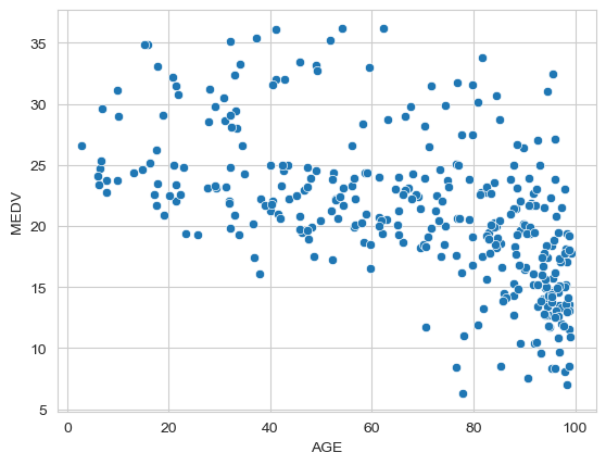
sns.histplot(filtered_df, x='AGE',bins=50)<Axes: xlabel='AGE', ylabel='Count'>
sns.histplot(filtered_df, x='DIS',bins=24)<Axes: xlabel='DIS', ylabel='Count'>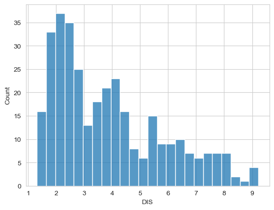
X = filtered_df.drop(['MEDV','RAD','TAX','CHAS'], axis = 1)
y = filtered_df['MEDV']
from sklearn.preprocessing import StandardScaler
ss = StandardScaler()
X_scaled = ss.fit_transform(X)X_train, X_test, y_train, y_test = train_test_split(X_scaled,y, test_size = 0.2, random_state=2024)lr.fit(X_train, y_train)
lr.score(X_test, y_test)0.8798651936746725y_pred_test2 = lr.predict(X_test)rmse2 = np.sqrt(mean_squared_error(y_test, y_pred_test2))rmse22.365310151851705