from sklearn.decomposition import PCA
from sklearn.preprocessing import StandardScaler
import pandas as pd
import numpy as np
import matplotlib.pyplot as plt
import seaborn as sns
CH9-08 PCA로 HAR데이터 분석
feature_url = 'https://raw.githubusercontent.com/PinkWink/ML_tutorial/master/dataset/HAR_dataset/features.txt'
features = pd.read_csv(feature_url,sep = '\s+', header = None, index_col = 0)
feature = list(features[1])
url = 'https://raw.githubusercontent.com/PinkWink/ML_tutorial/master/dataset/HAR_dataset/test/X_test.txt'
X_test = pd.read_csv(url, sep = '\s+', header = None)
url = 'https://raw.githubusercontent.com/PinkWink/ML_tutorial/master/dataset/HAR_dataset/test/y_test.txt'
y_test = pd.read_csv(url, sep = '\s+', header = None)url = 'https://raw.githubusercontent.com/PinkWink/ML_tutorial/master/dataset/HAR_dataset/train/X_train.txt'
X_train = pd.read_csv(url, sep = '\s+', header = None)
url = 'https://raw.githubusercontent.com/PinkWink/ML_tutorial/master/dataset/HAR_dataset/train/y_train.txt'
y_train = pd.read_csv(url, sep = '\s+', header = None)test_df = pd.concat([X_test,y_test], axis = 1)
train_df = pd.concat([X_train, y_train], axis = 1)test_df.columns = feature + ['actions']
train_df.columns = feature + ['actions']1. pca객체와 변환결과 반환하는 함수 정의하기
def transform_pca(X, n_components):
    pca = PCA(n_components=n_components, random_state=42)
    X_pca = pca.fit_transform(X)

return pca, X_pcapca, X_pca = transform_pca(X_train, 2)pca.mean_.shape(561,)pca.components_.shape(2, 561)pca.components_array([[-7.15326815e-05, -2.99847927e-04, -2.31385358e-04, ...,
-3.60833439e-02, 2.68253762e-02, 2.20742235e-02],
[ 3.25696388e-03, -4.22310901e-04, -8.39509411e-04, ...,
3.80396295e-02, -3.83432978e-02, -1.38720349e-02]])def get_df_pca(X_pca, y, cols):
temp_cols = [f'PCA_{col+1}' for col in range(cols.shape[0])]
df = pd.DataFrame(X_pca, columns = temp_cols)
df['actions'] = y
return dfdef get_pca_scores(pca):
print('pca_mean: ', pca.mean_)
print('설명된 분산: ', pca.explained_variance_)
print('설명된 분산비율합: ', np.sum(pca.explained_variance_ratio_))pca, X_pca = transform_pca(X_train, 2)
HAR_pca = get_df_pca(X_pca, y_train, pca.components_) HAR_pca.info()<class 'pandas.core.frame.DataFrame'>
RangeIndex: 7352 entries, 0 to 7351
Data columns (total 3 columns):
# Column Non-Null Count Dtype
--- ------ -------------- -----
0 PCA_1 7352 non-null float64
1 PCA_2 7352 non-null float64
2 actions 7352 non-null int64
dtypes: float64(2), int64(1)
memory usage: 172.4 KBHAR_pca.describe()| PCA_1 | PCA_2 | actions | |
|---|---|---|---|
| count | 7.352000e+03 | 7.352000e+03 | 7352.000000 |
| mean | -2.164874e-16 | 2.706093e-17 | 3.643362 |
| std | 5.901155e+00 | 1.653798e+00 | 1.744802 |
| min | -6.634712e+00 | -5.246209e+00 | 1.000000 |
| 25% | -5.572821e+00 | -1.176902e+00 | 2.000000 |
| 50% | -3.315931e+00 | 6.400354e-02 | 4.000000 |
| 75% | 5.638173e+00 | 1.145365e+00 | 5.000000 |
| max | 1.920990e+01 | 8.979156e+00 | 6.000000 |
HAR_pca.actions.unique()array([5, 4, 6, 1, 3, 2], dtype=int64)2. pairplot으로 pca1,pca2특성과 actions를 잘 구분했는지 보자
sns.pairplot(HAR_pca,hue='actions',height=5,aspect=1,palette='YlGnBu')<seaborn.axisgrid.PairGrid at 0x21f5efb5e10>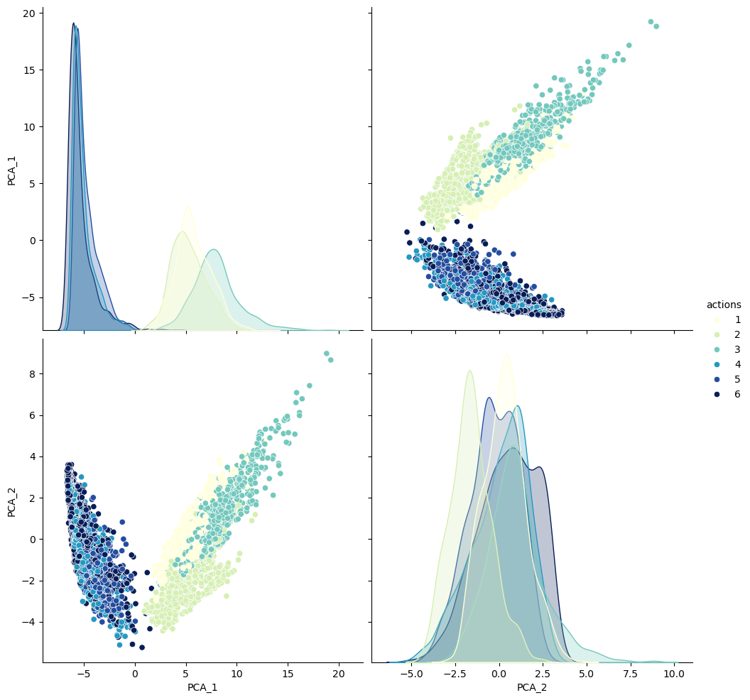
get_pca_scores(pca)설명된 분산: [34.82363041 2.73504627]
설명된 분산비율합: 0.67467462704879533. 주성분 10개 정도로 해보기
pca2,X_pca = transform_pca(X_train, 10)
HAR_pca2 = get_df_pca(X_pca, y_train, pca2.components_)HAR_pca2| PCA_1 | PCA_2 | PCA_3 | PCA_4 | PCA_5 | PCA_6 | PCA_7 | PCA_8 | PCA_9 | PCA_10 | actions | |
|---|---|---|---|---|---|---|---|---|---|---|---|
| 0 | -5.520280 | -0.290278 | -1.529929 | 1.333236 | 1.425096 | -0.194804 | 0.577301 | 0.691919 | -1.223694 | -0.365404 | 5 |
| 1 | -5.535350 | -0.082530 | -1.924804 | 0.671273 | 0.671266 | 0.735249 | -0.616831 | -0.771710 | -0.615282 | -0.894978 | 5 |
| 2 | -5.474988 | 0.287387 | -2.144642 | 0.531806 | 0.207850 | -0.037582 | 0.057787 | 0.094255 | -0.063200 | -0.219483 | 5 |
| 3 | -5.677232 | 0.897031 | -2.018220 | 0.157123 | 0.759086 | 1.079568 | -0.267829 | -0.731340 | 0.281281 | 0.466703 | 5 |
| 4 | -5.748749 | 1.162952 | -2.139533 | 0.207823 | 0.473049 | 0.462862 | -0.152459 | -0.108193 | 0.290587 | 0.543917 | 5 |
| ... | ... | ... | ... | ... | ... | ... | ... | ... | ... | ... | ... |
| 7347 | 6.253517 | -2.636767 | 0.448229 | 1.476510 | -0.767343 | -0.268674 | -1.349207 | -0.462989 | 1.461986 | 0.210340 | 2 |
| 7348 | 5.782321 | -2.437814 | 0.462731 | 1.711337 | -0.825479 | -0.404469 | -1.258027 | -0.318261 | 0.422658 | -0.816461 | 2 |
| 7349 | 5.857505 | -3.081843 | 0.671207 | 2.253643 | -0.494558 | 0.391464 | -1.000101 | -0.161922 | 0.290580 | 1.244097 | 2 |
| 7350 | 5.421095 | -3.426430 | 0.671243 | 2.013982 | -0.612627 | 0.442747 | -1.445923 | -0.112686 | 0.812234 | 1.681052 | 2 |
| 7351 | 5.497970 | -2.789929 | 0.005722 | 1.392948 | -0.805566 | -0.107339 | -0.923709 | -0.842863 | 0.997343 | 0.183705 | 2 |
7352 rows × 11 columns
get_pca_scores(pca2)설명된 분산: [34.82363041 2.73504627 2.29439284 1.04377529 0.943517 0.70815225
0.65505256 0.5950898 0.53964667 0.47764736]
설명된 분산비율합: 0.80503860456327034. 랜덤포레스트로 랜덤 서치 교차검증 돌려보기
from sklearn.model_selection import RandomizedSearchCV
from sklearn.ensemble import RandomForestClassifier
rf = RandomForestClassifier(random_state=42, verbose=1, n_jobs=-1)params = {
'max_depth' : range(2, 10),
'n_estimators' : [100, 200, 300],
}
rs = RandomizedSearchCV(rf, params, n_iter = 10, cv = 10)
rs.fit(HAR_pca2.drop('actions',axis=1), np.array(y_train).reshape(-1))print('cv_results: ',max(rs.cv_results_['mean_test_score']))cv_results: 0.8577275584146703print('best_params_: ', rs.best_params_)best_params_: {'n_estimators': 100, 'max_depth': 9}cv_df = pd.DataFrame(rs.cv_results_)cv_df[['rank_test_score','mean_test_score', 'params']]| rank_test_score | mean_test_score | params | |
|---|---|---|---|
| 0 | 3 | 0.850246 | {'n_estimators': 200, 'max_depth': 7} |
| 1 | 2 | 0.853918 | {'n_estimators': 100, 'max_depth': 8} |
| 2 | 7 | 0.823041 | {'n_estimators': 300, 'max_depth': 4} |
| 3 | 9 | 0.791073 | {'n_estimators': 200, 'max_depth': 3} |
| 4 | 1 | 0.857728 | {'n_estimators': 100, 'max_depth': 9} |
| 5 | 5 | 0.845350 | {'n_estimators': 300, 'max_depth': 6} |
| 6 | 6 | 0.835284 | {'n_estimators': 300, 'max_depth': 5} |
| 7 | 10 | 0.760332 | {'n_estimators': 100, 'max_depth': 2} |
| 8 | 4 | 0.845486 | {'n_estimators': 200, 'max_depth': 6} |
| 9 | 8 | 0.792569 | {'n_estimators': 100, 'max_depth': 3} |
5. rf 테스트데이터에 적용해보기
best_model = rs.best_estimator_get_pca_scores(pca2)설명된 분산: [34.82363041 2.73504627 2.29439284 1.04377529 0.943517 0.70815225
0.65505256 0.5950898 0.53964667 0.47764736]
설명된 분산비율합: 0.8050386045632703best_model.fit(HAR_pca2.drop('actions',axis=1), np.array(y_train).reshape(-1))
y_pred = best_model.predict(pca2.transform(X_test))from sklearn.metrics import classification_report, ConfusionMatrixDisplay
ConfusionMatrixDisplay.from_estimator(best_model, pca2.transform(X_test), y_test)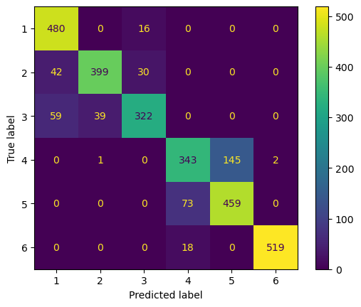
print(classification_report(y_test, y_pred, digits = 2)) precision recall f1-score support
1 0.83 0.97 0.89 496
2 0.91 0.85 0.88 471
3 0.88 0.77 0.82 420
4 0.79 0.70 0.74 491
5 0.76 0.86 0.81 532
6 1.00 0.97 0.98 537
accuracy 0.86 2947
macro avg 0.86 0.85 0.85 2947
weighted avg 0.86 0.86 0.85 29476. XGboost
np.unique(y_train)array([0, 1, 2, 3, 4, 5], dtype=int64)from sklearn.model_selection import train_test_split
X_sub, X_val, y_sub, y_val = \
train_test_split(HAR_pca2.drop('actions',axis=1), y_train, stratify = y_train,
test_size=0.2,random_state=42)print(X_sub.shape, y_sub.shape)
print(X_val.shape, y_val.shape)(5881, 10) (5881,)
(1471, 10) (1471,)X_val| PCA_1 | PCA_2 | PCA_3 | PCA_4 | PCA_5 | PCA_6 | PCA_7 | PCA_8 | PCA_9 | PCA_10 | |
|---|---|---|---|---|---|---|---|---|---|---|
| 3549 | 5.588663 | -0.363570 | 0.001601 | -1.629643 | -0.998808 | 0.168353 | -0.874047 | 0.589097 | -0.121209 | 0.839942 |
| 5608 | 5.464434 | 0.766964 | -0.392396 | -1.209731 | -0.372161 | 0.420398 | -0.336710 | -0.094319 | -0.667518 | -0.787488 |
| 5342 | -4.063030 | -1.559900 | 3.129090 | -1.236542 | -0.732668 | 0.378266 | 0.156751 | 0.525997 | 1.053626 | -0.528811 |
| 5450 | 2.933283 | -3.083015 | -0.068214 | 0.334995 | -0.409603 | -0.431156 | -1.086638 | -0.342928 | 0.678987 | 0.994511 |
| 3749 | 8.906528 | 2.665659 | -0.087004 | -0.399582 | 0.947653 | 1.152953 | -0.364983 | 0.099054 | -1.208306 | -0.975685 |
| ... | ... | ... | ... | ... | ... | ... | ... | ... | ... | ... |
| 6373 | 4.446453 | -0.314126 | -0.774878 | -1.298897 | -0.666031 | 0.124319 | -0.081351 | -0.147194 | -0.581189 | 1.501868 |
| 3332 | -6.149106 | 1.047273 | 2.335084 | 0.279198 | 0.170604 | -0.152179 | -0.171251 | 0.541352 | -0.377449 | 0.398390 |
| 3327 | -2.444945 | -1.877854 | 2.932734 | -1.313402 | -0.573453 | 0.434402 | 0.863757 | -0.929029 | 0.362572 | -0.727630 |
| 6666 | -5.460070 | 0.690586 | -0.529794 | -0.303853 | -0.403050 | 0.113865 | -0.619463 | -0.084114 | 0.726674 | 0.044042 |
| 2494 | 5.555998 | -0.797781 | 0.433985 | 1.758689 | -2.112869 | -0.300266 | -0.398123 | -0.197471 | -0.179571 | 0.675757 |
1471 rows × 10 columns
from xgboost import XGBClassifierxgb1 = XGBClassifier(random_state=42,n_jobs=-1, n_estimators = 500, learning_rate=0.123,)eval_set = [(X_val, y_val)]np.unique(y_sub)array([0, 1, 2, 3, 4, 5], dtype=int64)np.unique(y_val)array([0, 1, 2, 3, 4, 5], dtype=int64)xgb1.fit(X_sub, y_sub.values.reshape(-1),
eval_set = eval_set,early_stopping_rounds=10,) y_pred_val = xgb1.predict(X_val)print(classification_report(y_val, y_pred_val)) precision recall f1-score support
0 0.97 0.96 0.97 245
1 0.99 0.96 0.97 215
2 0.93 0.97 0.95 197
3 0.81 0.79 0.80 257
4 0.82 0.84 0.83 275
5 0.99 0.99 0.99 282
accuracy 0.92 1471
macro avg 0.92 0.92 0.92 1471
weighted avg 0.92 0.92 0.91 1471ConfusionMatrixDisplay.from_predictions(y_val, y_pred_val)<sklearn.metrics._plot.confusion_matrix.ConfusionMatrixDisplay at 0x21f0586b110>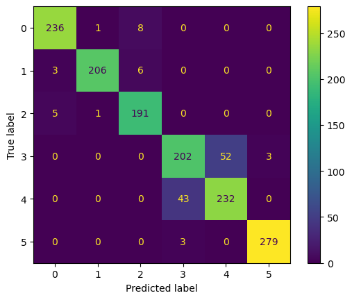
7. XGBoost를 테스트데이터에 적용한 결과
xgb2 = XGBClassifier(random_state=42,n_jobs=-1, n_estimators = 500, learning_rate=0.123, max_depth =10)xgb2.fit(HAR_pca2.drop('actions',axis=1), y_train)
y_pred = xgb2.predict(pca2.transform(X_test))print(classification_report(y_test, y_pred)) precision recall f1-score support
0 0.86 0.96 0.91 496
1 0.89 0.87 0.88 471
2 0.90 0.80 0.85 420
3 0.79 0.74 0.76 491
4 0.79 0.86 0.82 532
5 1.00 0.96 0.98 537
accuracy 0.87 2947
macro avg 0.87 0.87 0.87 2947
weighted avg 0.87 0.87 0.87 2947ConfusionMatrixDisplay.from_predictions(y_test, y_pred)<sklearn.metrics._plot.confusion_matrix.ConfusionMatrixDisplay at 0x21f021d7fd0>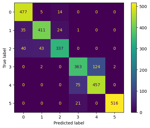
CH9-09 MNIST using PCA
import numpy as np
import matplotlib.pyplot as plt
import torch #파이토치 기본모듈
import torch.nn as nn
from torchvision import transforms, datasets
if torch.cuda.is_available():
DEVICE = torch.device('cuda') #GPU이용
else:
DEVICE = torch.device('cpu') #GPU이용안되면 CPU이용
print('Using PyTorch version:', torch.__version__, ' Device:', DEVICE)Using PyTorch version: 2.3.0.dev20240225 Device: cudatrain_dataset = datasets.MNIST(root ="../data/MNIST",
train = True,
download = True,
transform = transforms.ToTensor( ))
test_dataset = datasets.MNIST(root ="../data/MNIST",
train = False,
transform = transforms.ToTensor( ))# 먼저 CPU로 이동
train = train_dataset.data.cpu()
# 이제 NumPy 배열로 변환
train = train.numpy()test = test_dataset.data.cpu()
test = test.numpy()train.shape(60000, 28, 28)test.shape(10000, 28, 28)target_train = train_dataset.train_labels.cpu().numpy()target_test = test_dataset.test_labels.cpu().numpy()C:\Users\kd010\miniconda3\Lib\site-packages\torchvision\datasets\mnist.py:70: UserWarning: test_labels has been renamed targets
warnings.warn("test_labels has been renamed targets")target_trainarray([5, 0, 4, ..., 5, 6, 8], dtype=int64)target_testarray([7, 2, 1, ..., 4, 5, 6], dtype=int64)1. 데이터프레임 X_train, X_test 나누기
train_df = pd.DataFrame(train.reshape(60000,-1))
train_df['labels'] = target_train
test_df = pd.DataFrame(test.reshape(10000,-1))
test_df['labels'] = target_testtrain_dfX_train = train_df.drop('labels',axis=1)
X_test = test_df.drop('labels',axis=1)
y_train = train_df['labels']
y_test = test_df['labels']2. 16개 랜덤 초이스로 시각화하기
import randomnums = random.choices(range(60000), k=16)nums[26495,
14195,
3340,
12135,
1847,
34858,
13098,
22390,
25276,
57053,
9494,
49161,
19411,
9476,
32937,
7936]plt.figure(figsize=(12,12))
for idx, val in enumerate(nums):
plt.subplot(4, 4, idx+1)
plt.imshow(np.array(X_train.iloc[val,:]).reshape(28,28),cmap=plt.cm.Blues,)
plt.title(train_df.loc[val,'labels'])
plt.axis('off')
plt.grid(False)
plt.show()
CH9-10: MNIST데이터 KNN과 PCA로 학습
1. pipeline을 활용하여 pca로 차원축소 후 KNN으로 학습후 교차검증
from sklearn.preprocessing import StandardScaler
scaler = StandardScaler()
X_sc_train = scaler.fit_transform(X_train)
X_sc_test = scaler.transform(X_test)
from sklearn.pipeline import Pipeline
from sklearn.neighbors import KNeighborsClassifier
pipe = Pipeline([
('pca',PCA(random_state=42)),
('knn',KNeighborsClassifier())])
params = {
'pca__n_components':[3, 6, 10, 13],
'knn__n_neighbors':[5,10,15]
}from sklearn.model_selection import StratifiedKFold
skfold = StratifiedKFold(n_splits=10,shuffle=True,random_state=42)from sklearn.model_selection import RandomizedSearchCV
rmcv = RandomizedSearchCV(pipe, params, cv=skfold, n_jobs=-1,verbose=1,random_state=42)rmcv.fit(X_train, y_train)Fitting 10 folds for each of 10 candidates, totalling 100 fitsrmcv.best_params_{'pca__n_components': 13, 'knn__n_neighbors': 10}rmcv.cv_results_['mean_test_score'].max().round(4)0.9541rmcv.classes_array([0, 1, 2, 3, 4, 5, 6, 7, 8, 9], dtype=int64)y_tr_pred = rmcv.predict(X_train)print(classification_report(y_train, y_tr_pred)) precision recall f1-score support
0 0.98 0.99 0.98 5923
1 0.98 0.99 0.98 6742
2 0.97 0.97 0.97 5958
3 0.96 0.93 0.95 6131
4 0.97 0.95 0.96 5842
5 0.95 0.96 0.96 5421
6 0.97 0.99 0.98 5918
7 0.97 0.97 0.97 6265
8 0.96 0.93 0.95 5851
9 0.93 0.94 0.93 5949
accuracy 0.96 60000
macro avg 0.96 0.96 0.96 60000
weighted avg 0.96 0.96 0.96 60000ConfusionMatrixDisplay.from_predictions(y_train, y_tr_pred)<sklearn.metrics._plot.confusion_matrix.ConfusionMatrixDisplay at 0x21f1cab95d0>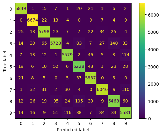
2. 랜덤서치로 찾은 best_model중에 random choice로 시각화해보기
nums = random.choices(range(60000), k=4)3. 실제 train 데이터
plt.figure(figsize=(12,12))
for idx, val in enumerate(nums):
    plt.subplot(2, 2, idx+1)
    plt.imshow(np.array(X_train.iloc[val,:]).reshape(28,28),
                        cmap=plt.cm.Blues,)
    plt.title(train_df.loc[val,'labels'])
    plt.axis('off')
    plt.grid(False)
plt.show()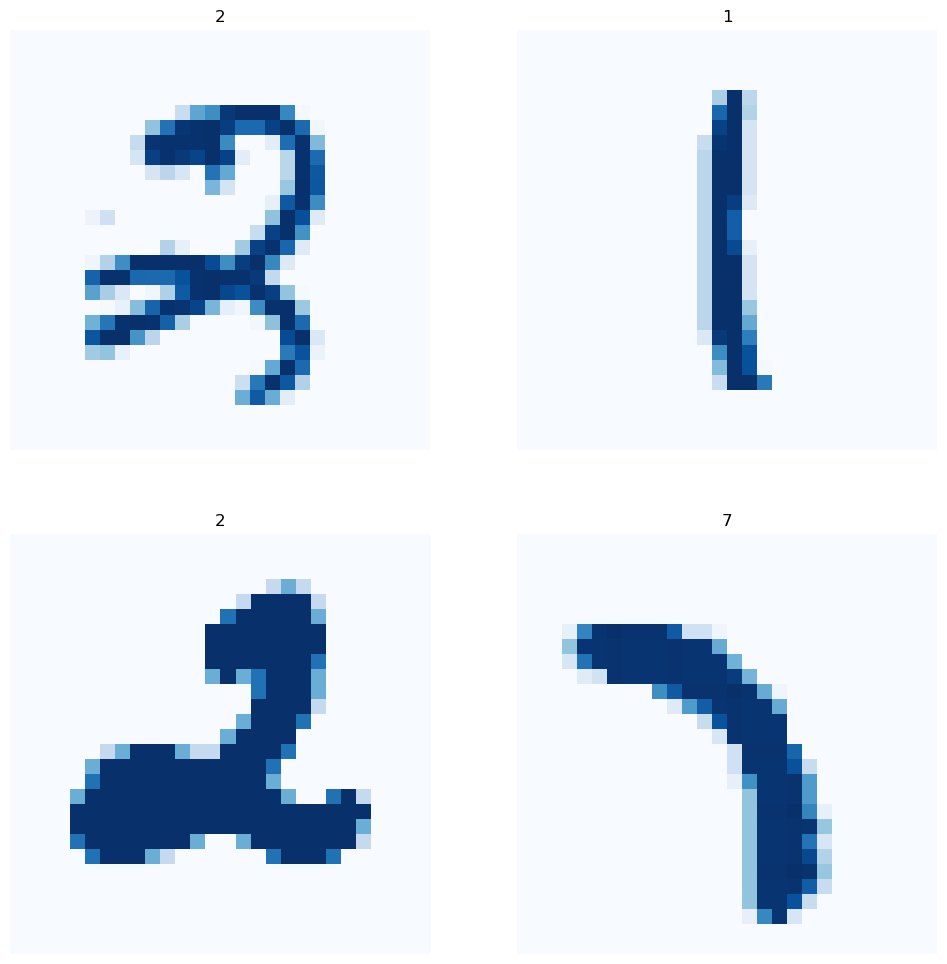
4. test데이터에 적용하여 성능 평가하기
y_test_pred = rmcv.best_estimator_.predict(X_test)print(classification_report(y_test, y_test_pred)) precision recall f1-score support
0 0.97 0.98 0.98 980
1 0.97 0.99 0.98 1135
2 0.96 0.96 0.96 1032
3 0.95 0.95 0.95 1010
4 0.96 0.95 0.95 982
5 0.94 0.94 0.94 892
6 0.96 0.98 0.97 958
7 0.96 0.93 0.95 1028
8 0.95 0.92 0.94 974
9 0.92 0.92 0.92 1009
accuracy 0.95 10000
macro avg 0.95 0.95 0.95 10000
weighted avg 0.95 0.95 0.95 10000ConfusionMatrixDisplay.from_predictions(y_test, y_test_pred)<sklearn.metrics._plot.confusion_matrix.ConfusionMatrixDisplay at 0x21f1ab34f50>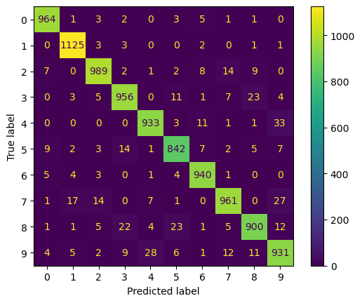
5. PCA 및 KNN으로 예측한 결과가 틀린것들을 무엇으로 예측했는지 보기
X_testy_test != y_test_pred0 False
1 False
2 False
3 False
4 False
...
9995 False
9996 False
9997 False
9998 False
9999 False
Name: labels, Length: 10000, dtype: boolwrong_ans = X_test[y_test != y_test_pred]wrong_ansnums = random.choices(population=wrong_ans.index, k=20)import koreanize_matplotlibplt.figure(figsize=(20,20))
for idx, val in enumerate(nums):
plt.subplot(4, 5, idx+1)
plt.imshow(np.array(wrong_ans.loc[val,:]).reshape(28,28),
cmap=plt.cm.Blues,)
plt.title(f'틀린예측: {y_test_pred[val]} \n 정답: {test_df.loc[val,"labels"]}',
fontsize=20)
plt.axis('off')
plt.grid(False)
plt.show()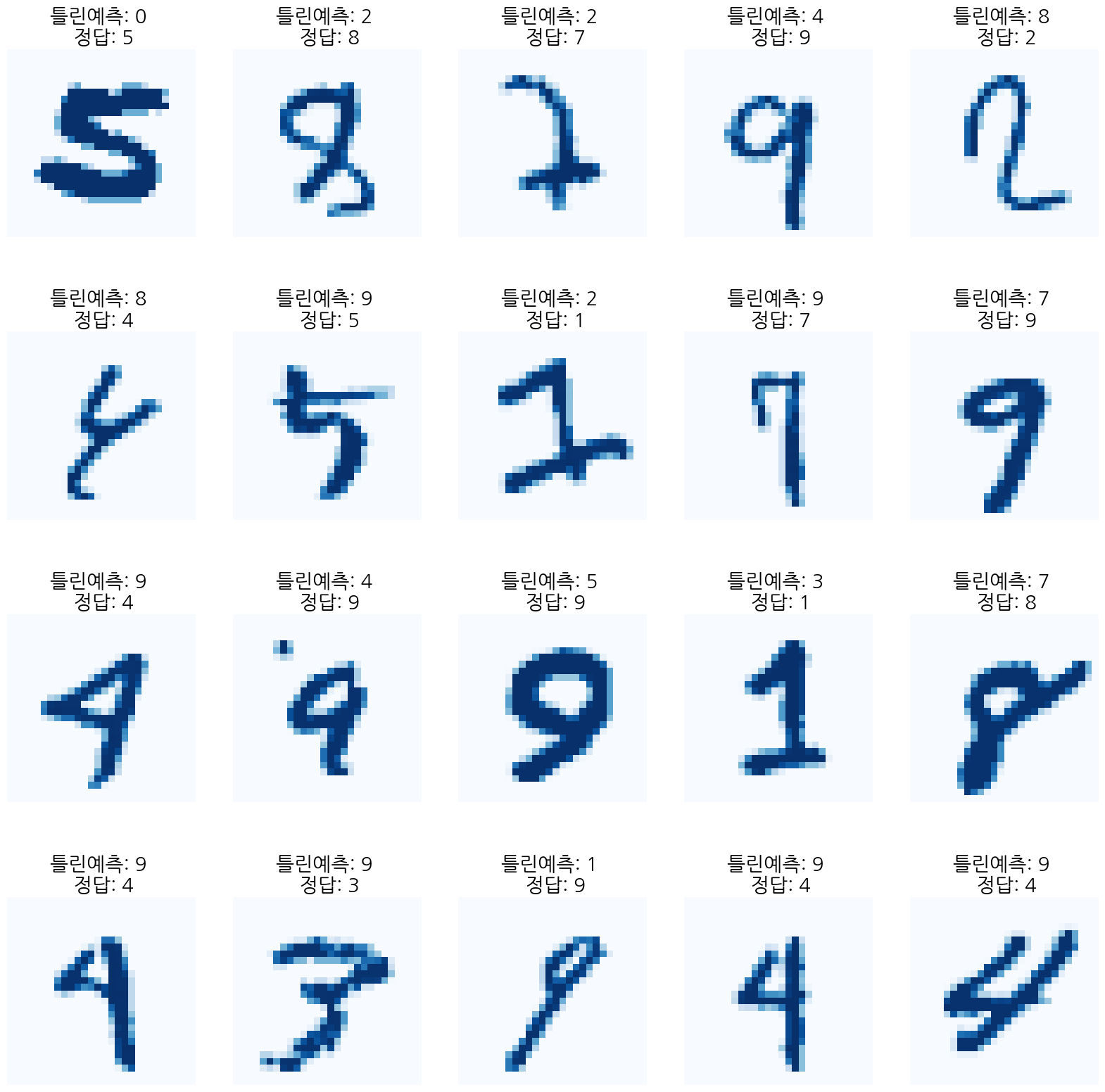
CH9-12: 네이머 북 서비스 API로 책가격 회귀분석
import urllib.request
import numpy as np
import pandas as pd
import datetime
import json
client_id =
client_secret =
def gen_search_url(api_node, search_text, start_num, disp_num):
base = 'https://openapi.naver.com/v1/search'
node = '/' + api_node +'.json'
param_query = '?query=' + urllib.parse.quote(search_text)
param_start = '&start=' + str(start_num)
param_disp = '&display=' + str(disp_num)
return base + node + param_query + param_disp + param_startdef get_result_onpage(url):
request = urllib.request.Request(url)
request.add_header('X-Naver-Client-Id', client_id)
request.add_header('X-Naver-Client-Secret', client_secret)
response = urllib.request.urlopen(request)
print('[%s] url Request Success' % datetime.datetime.now())
return json.loads(response.read().decode('utf-8'))url = gen_search_url('book', '머신러닝', 1, 100)
search_res = get_result_onpage(url)[2024-02-28 22:36:26.289985] url Request Successsearch_res['items'][50]{'title': 'AWS 머신러닝 마스터하기 (SageMaker, Apache Spark 및 TensorFlow를 사용한 Python의 고급 머신러닝)',
'link': 'https://search.shopping.naver.com/book/catalog/32492757397',
'image': 'https://shopping-phinf.pstatic.net/main_3249275/32492757397.20230722070902.jpg',
'author': 'Saket S. R. Mengle^Maximo Gurmendez',
'discount': '28500',
'publisher': 'DK로드북스',
'pubdate': '20201007',
'isbn': '9791196965648',
'description': 'AWS는 데이터 과학자들이 다양한 머신 러닝 클라우드 서비스를 탐색할 수 있도록 새로운 혁신을 지속적으로 추진하고 있다. 이 책은 AWS에서 고급 머신 러닝 알고리즘을 배우고 구현하기 위한 포괄적인 참고 도서이다.\n\n\n\n이 책으로 공부하면서 알고리즘들을 Elastic MapReduce의 Apache Spark, SageMaker 및 TensorFlow를 사용하여 AWS에서 훈련, 튜닝 및 배포하는 방법에 관한 통찰력을 얻을 수 있을 것이다. XGBoost, 선형 모델, 인수분해(Factorization) 머신 및 딥 네트워크와 같은 알고리즘에 중점을 두는 동시에, 이 책에서는 실제 문제를 해결하는 데 도움이 되는 세부적인 실용적 애플리케이션뿐만 아니라 AWS의 개요도 제공한다. \n\n\n\n모든 실용적 애플리케이션에는 AWS에서 실행하는 데 필요한 모든 코드가 포함된 일련의 컴패니언 노트북이 포함되어 있다. 다음 몇 장에서는 스마트 분석 및 예측 모델링에서 감정(어감) 분석에 이르기까지 SageMaker 및 EMR 노트북을 사용하여 다양한 작업을 수행하는 방법을 배운다.'}len(search_res['items'])100# title, price, publisher, isbn, linkdef get_df(res):
title = []; price = []
publisher = []; isbn = []
link = []
for i in range(len(res)):
title.append(res[i]['title'].strip("'"))
price.append(res[i]['discount'].strip("'"))
publisher.append(res[i]['publisher'].strip("'"))
isbn.append(res[i]['isbn'].strip("'"))
link.append(res[i]['link'].strip("'"))
value = {'title':title,
'price':price,
'publisher':publisher,
'isbn':isbn,
'link':link}
df = pd.DataFrame(value)
return dfres = []
for i in range(1,341,50):
url = gen_search_url('book', '머신러닝', i, 50)
search_res = get_result_onpage(url)
res.extend(search_res['items'])
df = get_df(res)
df[2024-02-28 22:36:31.646737] url Request Success
[2024-02-28 22:36:31.872018] url Request Success
[2024-02-28 22:36:32.122516] url Request Success
[2024-02-28 22:36:32.365479] url Request Success
[2024-02-28 22:36:32.636246] url Request Success
[2024-02-28 22:36:32.741379] url Request Success
[2024-02-28 22:36:32.985378] url Request Success| title | price | publisher | isbn | link | |
|---|---|---|---|---|---|
| 0 | 핸즈온 머신러닝 (사이킷런, 케라스, 텐서플로 2로 완벽 이해하는 머신러닝, 딥러닝... | 51300 | 한빛미디어 | 9791169211475 | https://search.shopping.naver.com/book/catalog... |
| 1 | 가상 면접 사례로 배우는 머신러닝 시스템 설계 기초 | 23090 | 인사이트 | 9788966264353 | https://search.shopping.naver.com/book/catalog... |
| 2 | 혼자 공부하는 머신러닝+딥러닝 (구글 코랩으로 환경 설정 없이 실습 가능) | 22230 | 한빛미디어 | 9791162243664 | https://search.shopping.naver.com/book/catalog... |
| 3 | 머신 러닝 (데이터를 이해하는 알고리즘의 예술과 과학) | 0 | 비제이퍼블릭 | 9791186697092 | https://search.shopping.naver.com/book/catalog... |
| 4 | R을 활용한 머신러닝 (데이터 준비부터 모델 조정, 평가, 빅데이터 작업까지) | 43200 | 에이콘출판 | 9791161758145 | https://search.shopping.naver.com/book/catalog... |
| ... | ... | ... | ... | ... | ... |
| 336 | Microsoft Azure Machine Learning Studio를 활용한 머... | 24300 | 한티미디어 | 9788964213506 | https://search.shopping.naver.com/book/catalog... |
| 337 | 텐서플로우 2와 케라스를 이용한 고급 딥러닝 (SageMaker, Apache Sp... | 37800 | DK로드북스 | 9791196965655 | https://search.shopping.naver.com/book/catalog... |
| 338 | 파이썬 데이터 사이언스 핸드북 (IPython, Jupyter, NumPy, Pan... | 32490 | 위키북스 | 9791158394271 | https://search.shopping.naver.com/book/catalog... |
| 339 | 4차 산업혁명 시대의 핵심, ICT 기술별 연구개발 및 특허 동향 분석 (인공지능(... | 396000 | IRS Global | 9791190870184 | https://search.shopping.naver.com/book/catalog... |
| 340 | 파이썬 데이터 사이언스 핸드북 (IPython, Jupyter, NumPy, Pan... | 34200 | 위키북스 | 9791158390730 | https://search.shopping.naver.com/book/catalog... |
341 rows × 5 columns
df['isbn'].nunique()341df.info()<class 'pandas.core.frame.DataFrame'>
RangeIndex: 341 entries, 0 to 340
Data columns (total 5 columns):
# Column Non-Null Count Dtype
--- ------ -------------- -----
0 title 341 non-null object
1 price 341 non-null object
2 publisher 341 non-null object
3 isbn 341 non-null object
4 link 341 non-null object
dtypes: object(5)
memory usage: 13.4+ KBdf['price'].value_counts(normalize=True)price
0 0.099707
27000 0.061584
31500 0.058651
22500 0.046921
24300 0.038123
...
35000 0.002933
10000 0.002933
16930 0.002933
17820 0.002933
396000 0.002933
Name: proportion, Length: 99, dtype: float641. 아마도 396000과 0인 가격은 이상치같음 없애자(나중에 페이지 num까지 가져온 후에)
from bs4 import BeautifulSoup
import selenium
from selenium.webdriver.common.by import By
from tqdm import tqdm
import time
import re
page = urllib.request.urlopen(df['link'][5])
txt = BeautifulSoup(page, 'html.parser')
page_nums = txt.select('#book_section-info li div span')[0].text[:3] def get_page_nums(df):
res = []
for idx,row in tqdm(df.iterrows()):
page = urllib.request.urlopen(row['link'])
try:
txt = BeautifulSoup(page, 'html.parser')
page_nums_string = txt.select('#book_section-info li div span')[0].text
match = re.search(r'\d+', page_nums_string)
page_nums = match.group()
res.append(int(page_nums))
except:
print(f'Error!! url: {url}')
res.append(np.nan)
return respage1 = get_page_nums(df[0:100])34it [00:42, 2.30it/s]
Error!! url: https://openapi.naver.com/v1/search/book.json?query=%EB%A8%B8%EC%8B%A0%EB%9F%AC%EB%8B%9D&display=50&start=301
100it [01:12, 1.39it/s]df_n = df[:100]df_n['page_nums'] = page1
df_n.dropna(axis=0,inplace=True)
df_n['page_nums'] = df_n['page_nums'].astype('int')df_n| title | price | publisher | isbn | link | page_nums | |
|---|---|---|---|---|---|---|
| 0 | 핸즈온 머신러닝 (사이킷런, 케라스, 텐서플로 2로 완벽 이해하는 머신러닝, 딥러닝... | 51300 | 한빛미디어 | 9791169211475 | https://search.shopping.naver.com/book/catalog... | 1044 |
| 1 | 가상 면접 사례로 배우는 머신러닝 시스템 설계 기초 | 23090 | 인사이트 | 9788966264353 | https://search.shopping.naver.com/book/catalog... | 336 |
| 2 | 혼자 공부하는 머신러닝+딥러닝 (구글 코랩으로 환경 설정 없이 실습 가능) | 22230 | 한빛미디어 | 9791162243664 | https://search.shopping.naver.com/book/catalog... | 580 |
| 3 | 머신 러닝 (데이터를 이해하는 알고리즘의 예술과 과학) | 0 | 비제이퍼블릭 | 9791186697092 | https://search.shopping.naver.com/book/catalog... | 512 |
| 4 | R을 활용한 머신러닝 (데이터 준비부터 모델 조정, 평가, 빅데이터 작업까지) | 43200 | 에이콘출판 | 9791161758145 | https://search.shopping.naver.com/book/catalog... | 932 |
| ... | ... | ... | ... | ... | ... | ... |
| 95 | 머신러닝 실무 프로젝트 (실전에 필요한 머신러닝 시스템 설계, 데이터 수집, 효과 ... | 16200 | 한빛미디어 | 9791162240816 | https://search.shopping.naver.com/book/catalog... | 228 |
| 96 | Spark와 머신 러닝 (빅데이터 분석과 예측 모델 트레이닝을 위한) | 0 | 에이콘출판 | 9788960778061 | https://search.shopping.naver.com/book/catalog... | 408 |
| 97 | 머신러닝(2학기, 워크북포함) | 20770 | 한국방송통신대학교출판문화원 | 9788920043314 | https://search.shopping.naver.com/book/catalog... | 392 |
| 98 | 머신러닝 알고리즘 마스터 (기계학습 및 응용프로그래밍에 대한 개념 부팅) | 0 | 도서출판 홍릉(홍릉과학출판사) | 9791156007081 | https://search.shopping.naver.com/book/catalog... | 584 |
| 99 | AWS 클라우드 머신러닝 (머신러닝 기초부터 AWS SageMaker까지) | 31500 | 에이콘출판 | 9791161754833 | https://search.shopping.naver.com/book/catalog... | 636 |
99 rows × 6 columns
2. 페이지수와 가격의 관계 찾아보기
df_n = df_n[df_n['price'] != '0']df_n['price']=df_n['price'].astype(int)C:\Users\kd010\AppData\Local\Temp\ipykernel_43056\3825412286.py:1: SettingWithCopyWarning:
A value is trying to be set on a copy of a slice from a DataFrame.
Try using .loc[row_indexer,col_indexer] = value instead
See the caveats in the documentation: https://pandas.pydata.org/pandas-docs/stable/user_guide/indexing.html#returning-a-view-versus-a-copy
df_n['price']=df_n['price'].astype(int)import seaborn as sns
sns.regplot(data=df_n,x='page_nums',y='price')<Axes: xlabel='page_nums', ylabel='price'>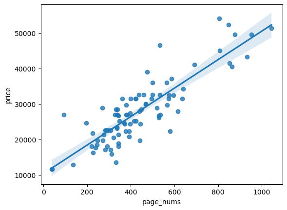
writer = pd.ExcelWriter('./ML_books.xlsx', engine='xlsxwriter')
df_n.to_excel(writer, sheet_name='Sheet1',index=False)

workbook = writer.book
worksheet = writer.sheets['Sheet1']
worksheet.set_column('A:A', 5)
worksheet.set_column('B:B', 60)
worksheet.set_column('C:C', 10)
worksheet.set_column('D:D', 15)
worksheet.set_column('F:F', 10)
worksheet.set_column('E:E', 50)
writer.close()
X = df_n['page_nums']
y = df_n['price']from sklearn.model_selection import train_test_split
X_train, X_test, y_train, y_test = train_test_split(X, y, test_size = 0.2, random_state=42)X_train56 344
69 414
80 848
76 576
83 384
...
22 196
67 528
78 396
16 332
58 586
Name: page_nums, Length: 72, dtype: int32from sklearn.linear_model import LinearRegression
lr = LinearRegression()
lr.fit(np.array(X_train).reshape(-1,1), np.array(y_train).reshape(-1,1))
y_test_pred = lr.predict(np.array(X_test).reshape(-1,1))y_test_predarray([[19253.17071872],
[23676.49853995],
[26046.13844418],
[23044.59456549],
[51638.24940986],
[27072.98240268],
[32997.08216325],
[42317.66578656],
[31417.3222271 ],
[24940.30648887],
[32681.13017602],
[23992.45052718],
[25256.2584761 ],
[28889.70632925],
[30153.51427818],
[19845.58069478],
[31575.29822071],
[26204.11443779]])from sklearn.metrics import mean_squared_error
mse = mean_squared_error(y_test,y_test_pred)
rmse = np.sqrt(mse)
print('mse', mse)
print('rmse', rmse)mse 20698603.95802392
rmse 4549.571843374267