[선형대수학] 행렬(2) - Product 및 선형변환

지난 포스팅 행렬(1) - 행렬의 정의 및 기본연산에 이어서 행렬의 곱셈(matrix multiplication), 선형변환(Linear Transformation)에 대해 알아보겠습니다.

matrix multiplication

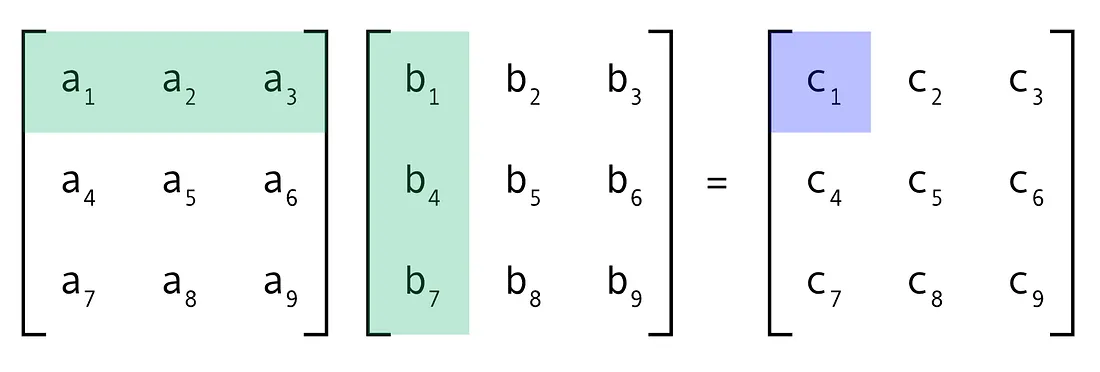
행렬의 곱셈 즉 행렬의 내적을 계산할 때는 위와 같이 "ㄱ"모양으로 진행하면 됩니다. 수식으로 설명하면 다음과 같습니다.

For $m \times n$ matrix $A$ and $n \times p$ matrix $B$,

위와 같이 행렬 A, B가 정의되어 있습니다. 그럼 $C = A\cdot B$는 다음과 같이 $m \times p$인 행렬이 됩니다.

다시 말해 $c_{ij}$는 $A$의 $i$번째 row vector(=$a_i$)와 $B$의 $j$번째 column vector(=$b_j$)의 내적으로 구할 수 있습니다.

example

sol>

import numpy as np

A = np.array([[1,0,2],
              [-1,3,1]])

B = np.array([[3,1],
              [2,1],
              [1,0]])


print(f"A\n{A}\n")

print(f"B \n {B}\n")

print(f"A x B \n {np.dot(A,B)}")

result

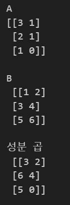
또한 numpy의 기능으로 행렬 각각의 성분 곱을 지원합니다. 이는 아래와 같습니다.

import numpy as np

A = np.array([[3,1],
              [2,1],
              [1,0]])


B = np.array([[1,2],
              [3,4],
              [5,6]])


print(f"A\n{A}\n")

print(f"B \n {B}\n")

print(f"성분 곱 \n {A * B}")

result

근데 만약 크기가 다른 행렬을 성분 곱을 취했을 때는 다음과 같은 Error가 발생합니다.

행렬과 벡터를 연산하는 데 있어서 size를 중요하게 고려해야합니다.

지금까지 행렬의 곱셈에 대해 설명하고 예제를 손으로 직접 구해도 보고 numpy를 이용해 구해봤습니다. 이제 부터는 행렬의 곱셈의 성질에 대해 알아보겠습니다.

Property1. Associativity

Let $A$ be a $m \times n$ matrix & $B$ be a $n \times p$ matrix & $C$ be a $p \times q$ matrix.
we have that

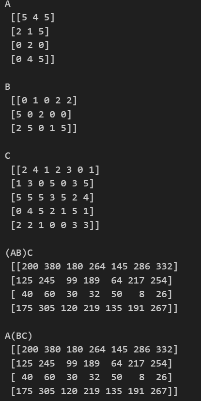
example> numpy를 이용해 무작위로 행렬을 만들고 값을 비교해보겠습니다.

Let $A$ be a $4 \times 3$ matrix & $B$ be a $3 \times 5$ matrix & $C$ be a $5 \times 7$ matrix.

import numpy as np

A = np.random.randint(6, size=(4,3))

B = np.random.randint(6, size=(3,5))

C = np.random.randint(6, size=(5,7))

print(f"A \n {A}\n")

print(f"B \n {B}\n")

print(f"C \n {C}\n")

m1 = np.dot(np.dot(A,B),C)

m2 = np.dot(A, np.dot(B,C))

print(f"(AB)C \n {m1}\n")

print(f"A(BC) \n {m2}\n")

result>

Property 2. distributivity

Let $A$ and $B$ be $m \times n$ matrices & $C$ be a $n \times p$ matrix.
we have that

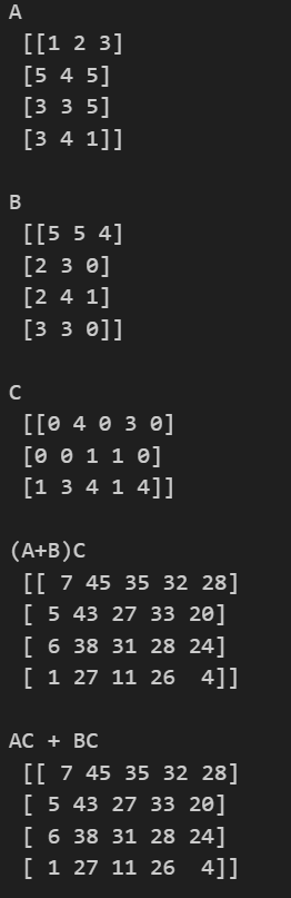
example> numpy를 이용해 무작위로 행렬을 만들고 값을 비교해보겠습니다.

Let $A$ and $B$ be $4 \times 3$ matrices & $C$ be a $3 \times 5$ matrix

import numpy as np

A = np.random.randint(6, size=(4,3))

B = np.random.randint(6, size=(4,3))

C = np.random.randint(6, size=(3,5))

print(f"A \n {A}\n")

print(f"B \n {B}\n")

print(f"C \n {C}\n")

r1 = np.dot((A + B),C)

r2 = np.dot(A,C) + np.dot(B,C)

print(f"(A+B)C \n {r1}\n")


print(f"AC + BC  \n {r2}\n")

result>

당연하게도 다음도 성립합니다.

Let $C$ be a $m \times n$ matrix & $A$ and $B$ be $n \times p$ matrices.
we have that

그리고 matrix multiplication에서는 교환법칙(commutative)이 성립되지 않습니다.

commutative ? $\Rightarrow$ 성립 x

당연하게 $A$가 $a \times b$ matrix이고 $B$가 $b \times c$ matrix 이면 애초에 행렬간의 곱셈을 취할 수 없습니다.
그리고 $A, B$가 $n \times n$인 정방 행렬인 경우에 대해서 살펴보겠습니다.

Let $AB = C$ and $BA = C^{\ \prime}$. and we have that

So$\quad c_{ij} \ne c_{ij}^{\ \prime} \quad \Rightarrow \quad C \ne C^{\ \prime}.$

일반적으로 행렬의 곱셈에서 교환법칙은 성립하지 않습니다.

Row Operation(기본 행 연산)과 Linear equations(방정식)에 대해서는 다음에 다루도록 하겠습니다.

이제는 Linear Transformations(선형변환)에 대해 알아보겠습니다.

Linear Transformations

간단하게 선형 변환은 차원을 늘리거나 축소시키는 것을 의미합니다.
먼저 수학적으로 정의부터 살펴보겠습니다.

Def> linear transformation

Let $V, W$ be vector spaces over the same field $F$.
A function $T : V \rightarrow W$ is said to be a linear transformation if for any two vectors $u, v \in V$ and any scalar $k \in F$ the following two conditions ar satisfied:

• additivity : $T(u + v) = T(u) + T(v)$
• homogeneity : $T(ku) = k T(u)$
• $T(ku+v) = kT(u) + T(v)$

위키 백과를 통한 수학적 정의는 위와 같습니다. 예제를 들어 설명해보겠습니다.

example>
Let $A$ be a $m \times n$ matrix

즉 위에서는 $n$차원인 $u$ 벡터가 $m$ 차원인 $v$ 벡터로 선형변환 된것입니다.

선형변환은 이후 차원 축소, 차원 확대, 고유값 고유벡터를 설명할 때 쓰이는 아주 중요한 개념 입니다.

추가적으로 더 궁금한 내용이나 포스팅에 오류가 있을 경우 댓글 부탁드립니다. 이번 포스팅은 여기서 마치겠습니다.

Reference

• https://ko.wikipedia.org/wiki/%ED%96%89%EB%A0%AC

• https://en.wikipedia.org/wiki/Matrix_(mathematics)

• https://en.wikipedia.org/wiki/Matrix_multiplication

• https://charchithowitzer.medium.com/matrix-multiplication-why-is-it-a-big-deal-cc8ef7490008

• https://numpy.org/doc/stable/reference/random/generated/numpy.random.randn.html

• https://en.wikipedia.org/wiki/Elementary_matrix