(2020)Denoising Diffusion Probabilistic Models

0. Abstract

본 논문은 nonequilibrium thermodynamics로 부터 영감을 받은 latent variable을 이용하는 diffusion probabilistic models로 hight quality의 image synthesis를 얻었다.

Diffusion probabilistic models와 Langevin dynamics의 denoising score matching간의 novel connection에 따라 설계된 weighted variational bound로 부터 가장 좋은 결과를 얻었으며 본 논문의 models는 autoregressive decoding로 볼 수 있는 progressive lossy decompression을 인정한다.

CIFAR10에서 Inception score와 FID로 SOTA를 달성하였으며 LSUN에서 ProgressiveGAN과 동등한 quality를 얻었다.

1. Introduction

GANs, autoregressive models, flows, VAEs는 image와 audio synthesize에서 놀라운 성능을 보여준다. 그리고 GANs에 견줄만한 energy-based modeling과 score matching 방법들의 발전이 있었다.

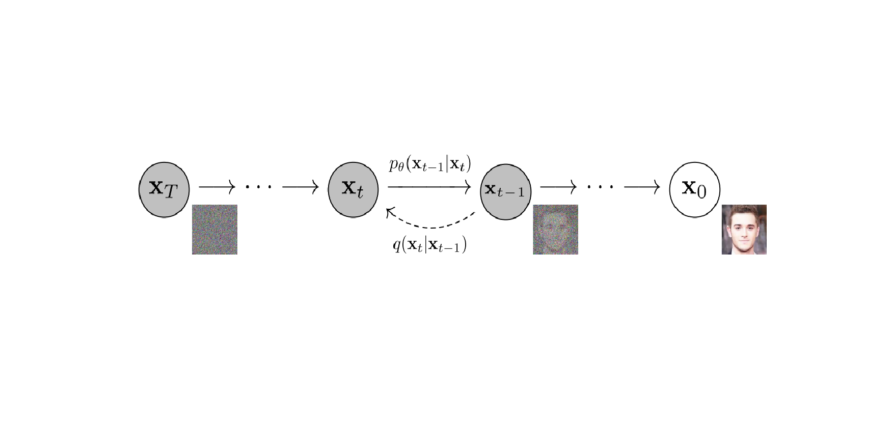
본 논문은 diffusion probabilitics models의 progress를 제안한다. Diffusion model은 유한한 시간 이후에 data와 일치하는 sample을 생성을 하기 위해 variational inference를 사용하여 parameterized Markov chain을 학습한다.

Diffusion models는 정의하기가 쉽고 효율적인 학습이 가능하나 이 모델이 hight quality의 samples를 생성할 수 있다는 것을 입증할 수 없다. 결과를 봤을 때 이전에 제안이 된 연구들 보다 좋은 결과를 보여줌을 확인할 뿐이다.

또한, multiple noise levels에 대한 denoising score matching은 sampling 중 참조된 Langevin dynamics와 동등함을 보여준다. 이러한 특징이 hight quality의 samples를 얻는데 큰 기여를 했다고 예상을 해볼 수는 있다.

그럼에도 불구하고 본 논문의 model은 다른 likelihood 기반의 model들과 비교했을 때 적절한 log likelihoods를 갖고 있지 않다. 그러나 본 논문에서는 loss compression이라는 언어로 정확한 분석을 제시하고 diffusion models의 sampling 과정이 autoregressive decoding과 유사한 progressive decoding임을 보여준다.

2. Background

Diffusion models는 latent variable models이다. $\text{x}_1,\ \ldots\ ,\ \text{x}_T$는 $\text{x}_0\ \sim\ q(\text{x}_0)$와 같은 dimensionality를 갖는 latents이다. $p_\theta(\text{x}_{0:T})$는 reverse process라고 부르며, $p(\text{x}_T)=\mathcal{N}(\text{x}_T;0,\text{I})$에서 시작하는 학습된 Gaussian transitions의 Markov chain이다.

$p_\theta(\text{x}_{0:T}):=p(\text{x}_T)\prod\limits_{t=1}^Tp_{\theta}(\text{x}_{t-1}|\text{x}_t)$

$p_{\theta}(\text{x}_{t-1}|\text{x}_t):=\mathcal{N}(\text{x}_{t-1};\mu_{\theta}(\text{x}_t,t),\sum_{\theta}(\text{x}_t,t))$

다른 type의 latent variable models와 다른 점은 posterior $q(\text{x}_{1:T}|\text{x}_0)$을 approximate 한다는 것이다. 이를 forward process 또는 diffusion process로 불리며 $\beta_1,\ldots,\beta_T$의 variance schedule을 따르는 Gaussian noise를 점진적으로 더한 Markov chain에 의해 고정된다.

$q(\text{x}_{1:T}|\text{x}_0):=\prod\limits_{t=1}^Tq(\text{x}_t|\text{x}_{t-1})$

$q(\text{x}_t|\text{x}_{t-1}):=\mathcal{N}(\text{x}_t;\sqrt{1-\beta_t}\text{x}_{t-1},\beta_t\text{I})$

학습은 negative log likelihood의 usual variational bound를 optimize 한다.

$\mathbb{E}[-\log p_{\theta}(x_0)]\leq\mathbb{E}_q\left[-\log\cfrac{p_\theta(\text{x}_{0:T})}{q(\text{x}_{1:T}|\text{x}_0)}\right]=$

$\mathbb{E}_q\left[-\log_p(\text{x}_T)-\sum\limits_{t\geq1}\log\cfrac{p_\theta(\text{x}_{t-1}|\text{x}_t)}{q(\text{x}_t|\text{x}_{t-1})}\right]=:L$

Forward process의 variances $\beta_t$는 reprameterization에 의해 학습될 수도 있고 hyperparameters와 같이 constant가 될 수도 있다. 그리고 reverse process는 $p_{\theta}(\text{x}_{t-1}|\text{x}_t)$에서 Gaussian conditionals의 선택에 의해 expressiveness가 보장이 된다. 왜냐하면 $\beta_t$가 매우 작을 때, 같은 functional form을 두 process가 갖기 때문이다. Forward process의 중요한 특징은 임의의 timestep $t$에서 closed form으로 sampling $\text{x}_t$를 허용한다는 점이다.

$\alpha_t=:1-\beta_t,\ \bar{\alpha}_t=:\prod_{s=1}^t\alpha_s$

$q(\text{x}_t|\text{x}_0)=\mathcal{N}(\text{x}_t;\sqrt{\bar{\alpha}}\text{x}_0,\ (1-\bar{\alpha_t})\text{I}$

따라서 stochastic gradient descent로 $L$의 random terms를 optimize하여 효율적인 학습이 가능하다. $L$을 다음과 같이 작성하여 variance reduction에서 추가적인 개선이 있다.

$\mathbb{E}_q\left[\underbrace{D_{\text{KL}}(q(\text{x}_T|\text{x}_0)||p(\text{x}_T))}_{L_t}+\sum\limits_{t>1}\underbrace{D_{\text{KL}}(q(\text{x}_{t-1}|\text{x}_t,\text{x}_0)||p_{\theta}(\text{x}_{t-1}|\text{x}_t))}_{L_{t-1}}\underbrace{-\log p_{\theta}(\text{x}_0|\text{x}_1)}_{L_0}\right]$

위 식은 KL divergence를 사용하여 $\text{x}_0$가 주어졌을 때 다루기가 수월한 forward process posteriors와 $p_\theta(\text{x}_{t-1}|\text{x}_t)$를 직접 비교한다. posteriors $q$에 관한 식은 아래와 같다.

$q(\text{x}_{t-1}|\text{x}_t,\text{x}_0)=\mathcal{N}(\text{x}_{t-1};\tilde{\mu}_t(\text{x}_t,\text{x}_0),\tilde{\beta}_t\text{I}),$

$\text{where}\ \ \tilde{\mu}_t(\text{x}_t,\text{x}_0):=\cfrac{\sqrt{\bar{\alpha}_{t-1}}\beta_t}{1-\bar{\alpha}_t}\text{x}_0+\cfrac{\sqrt{\alpha_t}(1-\bar{\alpha}_{t-1})}{1-\bar{\alpha}_t}\text{x}_t\ \ \text{and}\ \ \tilde{\beta}_t:=\cfrac{1-\bar{\alpha}_{t-1}}{1-\bar{\alpha}_t}\beta_t$

KL divergences는 모두 Gaussians간의 비교이므로 high variance Monte Carlo estimates 대신에 closed form expressions의 Rao-Blackwellized 방식으로 계산할 수 있다.

3. Diffusion models and denoising autoencoders

Diffusion models는 latent models의 제한된 한 종류처럼 보이지만 구현 시 많은 자유도를 갖고 있다. 가장 먼저 정해야 할 것은 forward process의 분산 $\beta_t$와 reverse process의 model architecture, 그리고 Gaussian distribution parameterization이다. 이를 살펴보기 위해 본 논문에서는 diffusion models와 denoising score matching간의 연결을 설명한다. 궁극적으로, 본 논문의 model은 simplicity와 emprical results로 design이 된다.

3.1 Forward process and $L_T$

Forward process의 분산 $\beta_t$를 reprameterization으로 학습을 하는 대신 constant로 고정한다. 따라서 구현 시, approximate posterior $q$는 학습이 가능한 parameters가 아니고 $L_T$는 학습하는 동안 constant 이므로 무시가 가능하다.

3.2 Reverse process and $L_{1:T-1}$

다음으로 $p_{\theta}(\text{x}_{t-1}|\text{x}_t)=\mathcal{N}(\text{x}_{t-1};\mu_{\theta}(\text{x}_t,t),\sum_{\theta}(\text{x}_t,t))$에 대해 살펴본다. 첫 번째로, time dependent constant로 제한하기 위해서 $\sum_\theta(\text{x},t)=\sigma_t^2\text{I}$로 설정하였다. 실험을 해보았을 때, $\sigma^2=\beta_t$와 $\sigma^2=\tilde{\beta}_t=\frac{1-\bar{\alpha}_{t-1}}{1-\bar{\alpha}_t}\beta_t$는 비슷한 결과를 얻었다. 이는 $\text{x}_0\sim\mathcal{N}(0,\text{I})$이고 $\text{x}_0$이 one point로 설정했을 때 최적이다.

두 번째로, 평균 $\mu_\theta(\text{x}_t,t)$을 나타내기 위해서 $L_t$식을 따라 구체적인 parameterization을 제안한다.

$L_{t-1}=\mathbb{E}_q\left[\cfrac{1}{2\sigma_t^2}||\tilde{\mu}_t(\text{x}_t,\text{x}_0)-\mu_{\theta}(\text{x}_t,t)||^2\right]+C$

$C$는 constant이며 $\theta$에 영향을 받지 않는다. 즉, $\mu_\theta$의 parameterization은 forward process posterior의 평균인 $\tilde{\mu}_t$를 예측하는 model과 같다.

그러나 식 $q(\text{x}_t|\text{x}_0)=\mathcal{N}(\text{x}_t;\sqrt{\bar{\alpha}}\text{x}_0,\ (1-\bar{\alpha_t})\text{I}$과 forward process의 posterior formula를 적용해 다음과 같이 식을 확장할 수 있다.

$L_{t-1}-C$

$=\mathbb{E}_{\text{x}_0,\epsilon}\left[\cfrac{1}{2\sigma_t^2}\left|\left|\tilde{\mu}_t\left(\text{x}_t(\text{x}_0,\epsilon),\cfrac{1}{\sqrt{\bar{\alpha}_t}}(\text{x}_t(\text{x}_0,\epsilon)-\sqrt{1-\bar{\alpha}_t}\epsilon)\right)-\mu_{\theta}(\text{x}_t(\text{x}_0,\epsilon),t)\right|\right|^2\right]$

$=\mathbb{E}_{\text{x}_0,\epsilon}\left[\cfrac{1}{2\sigma_t^2}\left|\left|\cfrac{1}{\sqrt{\alpha}_t}\left(\text{x}_t(\text{x}_0,\epsilon)-\cfrac{\beta_t}{\sqrt{1-\bar{\alpha}}_t}\epsilon\right)-\mu_\theta(\text{x}_t(\text{x}_0,\epsilon),t)\right|\right|^2\right]$

위 식을 통해 $\mu_{\theta}$는 $\text{x}_t$가 주어진 $\frac{1}{\sqrt{\alpha_t}}\left(\text{x}_t-\frac{\beta_t}{\sqrt{1-\bar{\alpha}}_t}\epsilon\right)$을 예측해야 하기 때문에 $\text{x}_t$는 model의 input이 될 수 있고 다음과 같이 parameterization할 수 있다.

$\mu_\theta(\text{t},t)=\tilde{\mu}_t\left(\text{x}_t,\cfrac{1}{\sqrt{\bar{\alpha}_t}}(\text{x}_t-\sqrt{1-\bar{\alpha}_t}\epsilon_\theta(\text{x}_t))\right)=\cfrac{1}{\sqrt{\alpha}_t}\left(\text{x}_t-\cfrac{\beta_t}{\sqrt{1-\bar{\alpha}_t}}\epsilon_\theta(\text{x}_t,t)\right)$

$\text{x}_{t-1}\sim p_\theta(\text{x}_{t-1}|\text{x})$을 얻기 위해서는 아래의 식을 계산해야 한다.

$\text{x}_{t-1}=\cfrac{1}{\sqrt{\alpha_t}}\left(\text{x}_t-\cfrac{\beta-t}{\sqrt{1-\bar{\alpha_t}}}\epsilon_\theta(\text{x}_t,t)\right)+\sigma_t\text{z},\ \ \text{where}\ \text{z}\sim\mathcal{N}(0,\text{I})$

요약하면, reverse process의 $\mu_\theta$를 학습해 $\tilde{\mu}$를 예측하거나 parameterization을 수정함으로 학습을 통해 $\epsilon$을 예측할 수 있다.

$\epsilon$-prediction parameterization은 Langevin dynamics와 유사하고 diffusion model의 variational bound를 simplify 한다는 것을 보여준다. 그러나 이것은 $p_{\theta}(\text{x}_{t-1}|\text{x}_t)$의 또 다른 parameterization일 뿐이며 본 논문에서는 $\tilde{\mu}_t$를 예측하는 것과 비교해서 ablantion study를 진행할 예정이다.

3.3 Data scaling, reverse process decoder, and $L_0$

Image data는 $\{0,1,\ldots,255\}$의 integers에서 $[-1,1]$로 scaled 된다고 가정한다. 이를 통해 reverse process의 neural network가 $p(\text{x}_T)$에서 시작하여 일관되게 scaled 된 input을 입력받을 수 있다. Discrete log likelihoods를 얻기 위해서 reverse process의 마지막 term을 Gaussian $\mathcal{N}(\text{x}_0;\mu_\theta(\text{x}_1,1),\sigma_1^2\text{I})$에서 얻은 독립적인 discrete decoder로 설정한다.

$p_{\theta}(\text{x}_0|\text{x}_1)={\displaystyle \prod\limits_{i=1}^D\int _{\delta-(x_0^i)}^{\delta+(x_0^i)}}\mathcal{N}(x;\mu_\theta^i(\text{x}_1,1),\sigma_1^2)dx$

$\delta_+(x)= \begin{cases} \infin &\text{if}\ x=1 \\ x+\frac{1}{255} &\text{if}\ x<1 \end{cases}\ \ \ \ \ \ \ \ \delta_-(x)= \begin{cases} -\infin &\text{if}\ x=-1 \\ x-\frac{1}{255} &\text{if}\ x>-1 \end{cases}$

$D$는 data dimensionality이고 $i$는 coordinate를 나타낸다. VAE decoders와 autoregressive models에 사용되는 discretized continuous distributions와 같이 본 논문의 선택은 data에 noise를 추가하거나 scaling operation의 Jacobian을 log likelihood에 통합할 필요 없이 variational bound가 discrete data의 lossless condelength임을 보장한다. Sampling이 끝나면 noise 없이 $\mu_\theta(\text{x}_1,1)$을 표현한다.

3.4 Simplified training objective

위에서 정의한 reverse process, decoder, variational bound를 사용하여 $\theta$의 관점에서 명확하게 미분 가능하며 학습할 준비가 되었다. 그러나 다음과 같이 variational bound을 변형해 학습하는 것이 sample quality와 구현 측면에서 유리함을 발견했다.

$L_{\text{simple}}(\theta):=\mathbb{E}_{t,\text{x}_0,\epsilon}\left[||\epsilon-\epsilon_\theta(\sqrt{\bar{\alpha_t}\text{x}_0+\sqrt{1-\bar{\alpha}_t}}\epsilon)||^2\right]$

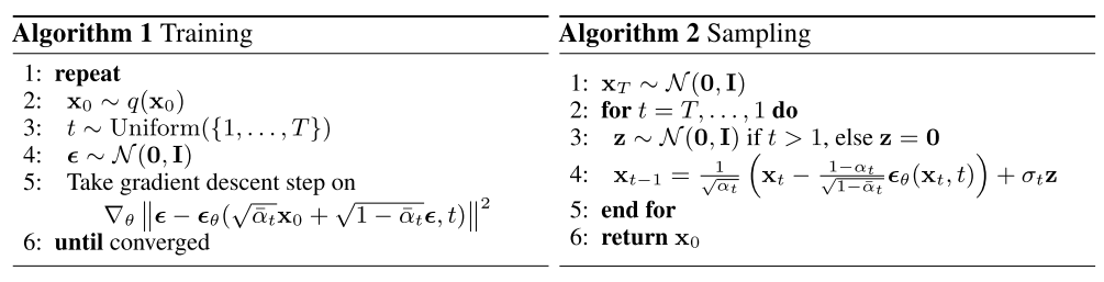
Algorithm 1은 위의 simplified objective로 전체 procedure를 나타내고 있으며 Algorithm 2는 data densitiy의 학습된 gradient로 $\epsilon_\theta$를 사용하며 Langevin dynamics와 유사하다.

4. Experiments

이전 연구들과 조건을 맞추기 위해서 $T=1000$으로 설정했다. 그리고 forward process의 분산을 $\beta_1=10^{-4}$에서 $\beta_T=0.02$로 설정했다.

Reverse process를 위해 unmasked PixelCNN++의 U-Net backbone을 group normalization과 함께 사용하였다. Parameters는 시간에 따라 공유되며, Transformer sinusoidal postion embedding을 사용하여 network에 적용된다. $16\times16$ feature map resolution에서 self-attention을 적용한다.

4.1 Sample quality

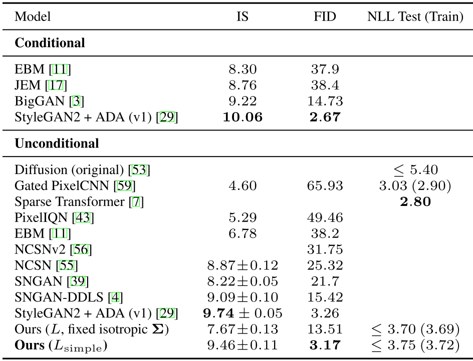
위 표는 CIFAR10에 대한 Inception scores, FID scores, log likelihoods를 보여준다. FID가 3.17인 본 논문의 model은 conditional models를 포함하여 대부분의 model보다 나은 samaple quality를 달성하였다.

4.2 Reverse process parameterization and training objective ablation

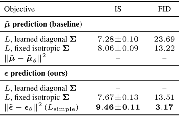
위 표는 reverse process의 parameterizations와 training objectives가 주는 sample quality에 대한 영향을 보여준다. $\tilde{\mu}$를 예측하는 baseline option은 unweighted mean squared error대신 true variational bound에 대해 학습된 경우에 좋은 성능을 얻을 수 있었다. 또한 reverse process에서 variances를 학습하면 fixed variances에 비해 불안정하고 낮은 sample quality를 얻었다. $\epsilon$를 예측하는 것은 본 논문에서 제안을 한 것처럼 fixed variances에서 variational bound에 대해 학습하는 것은 $\tilde{u}$를 예측하는 것을 근사화 할 뿐만 아니라 simplified objective로 학습할 때 더 좋다.

4.3 Progressive coding

위 첫 번째 표를 보면 train과 test간의 gap은 대략 0.03 bits/dimension이다. 이는 다른 likelihood-based models과 비교할 만하고 diffusion model이 overfitting하지 않음을 보여준다. 하지만 codelengths는 energy based models보다는 낫지만 likelihood based generative models보다는 경쟁력이 없다.

그럼에도 불구하고 sample quality가 높기 때문에 diffusion models는 훌륭한 lossy compressors를 만드는 inductive bias가 있다고 결론을 내렸다. Variational bound term $L_1+\cdots+L_T$를 rate, $L_0$를 distortion이라 할 때, CIFAR10 model은 1.78 bits/dim의 rate와 1.97 bits/dim의 distortion을 얻었으며 이 정도의 수치는 0-255 scale에서 0.95의 RMSE의 수치이다.

4.3.1 Progressive lossy compression

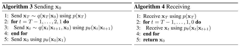
본 논문의 model의 ratio-distortion을 더 잘 보여주기 위해 progressive lossy code를 설명한다. Minimal random code와 같은 procedure들의 접근을 가정한 Algorithm 3, 4는 $q$와 $p$의 KL Divergence를 이용해 sample $\text{x}\sim q(\text{x})$를 transmit할 수 있고, 이 경우 receiver는 $p$만 사용할 수 있다. 이 경우에 Algorithm 3, 4는 $\text{x}_T,\ldots,\text{x}_0$을 순차적으로 transmit할 수 있다.

이때, 임의의 시간 $t$에서 receiver의 partial information인 $\text{x}_t$를 사용할 수 있으며 다음 식을 이용해 progressive하게 추정할 수 있다.

$\text{x}_0\approx\hat{\text{x}}_0=(\text{x}_t-\sqrt{1-\bar{\alpha}_t}\epsilon_\theta(\text{x}_t))/\sqrt{\bar{\alpha}_t}$

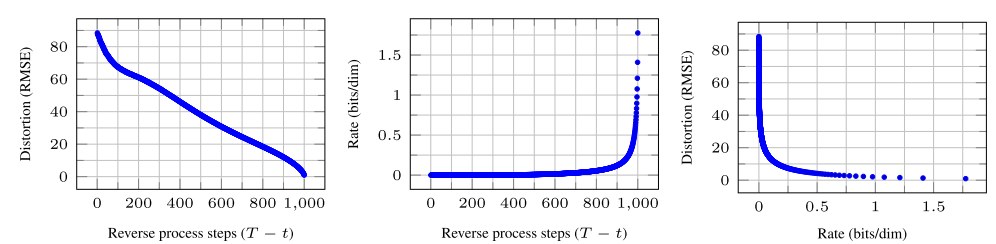
위 그림은 각 time $t$에서 distortion과 rate를 plot한 그래프이다. distortion은 $\sqrt{||\text{x}_0-\hat{\text{x}}_0||^2/D}$ 로 $\text{x}_0$와 $\text{x}_0$를 estimate한 값과의 RMSE를 계산했고, rate는 receivced 된 bit의 누적으로 계산했다고 한다. distortion은 distortion-rate plot에서 낮은 rate에서 빠르게 감소하는데 이를 통해 bit의 대부분이 imperceptible distortion에 존재함을 확인할 수다.

4.3.2 Progressive generation

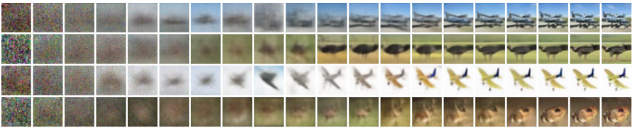
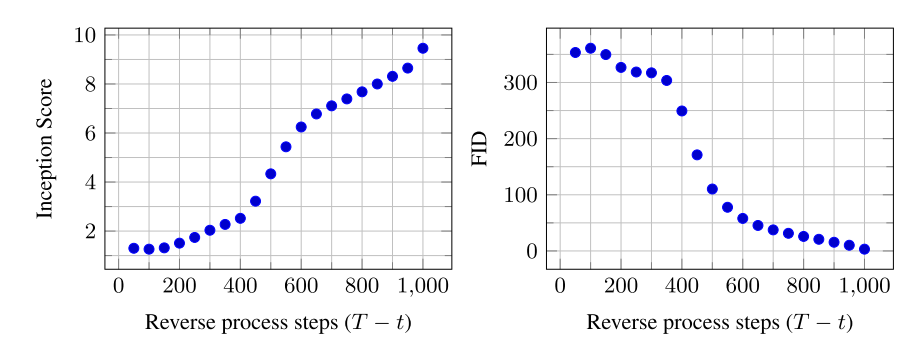
본 논문은 또한 random bits로 부터 progressive decompression에 의한 unconditional generation process를 수행하였다. 즉, Algorithm 2를 사용하여 reverse process의 sampling 과정에서 $\hat{\text{x}}_0$를 예측한다. 위 두 그림은 reverse proess에서 $\hat{\text{x}}_0$의 sample quality의 결과를 보여준다.

4.3.3 Connection to autoregressive decoding

Variational bound식을 다시 쓰면 다음과 같이 쓸 수 있다.

$L={D_{\text{KL}}(q(\text{x}_T)||p(\text{x}_T))}+\mathbb{E}_q\left[\sum\limits_{t>1}{D_{\text{KL}}(q(\text{x}_{t-1}|\text{x}_t)||p_{\theta}(\text{x}_{t-1}|\text{x}_t))}\right]+H(\text{x}_0)$

$q(\text{x}_t|\text{x}_0)$를 $\text{x}_0$의 $t$번째 coordinates로 정의해서 $T$를 데이터의 dimensionality으로 설정할 수 있다. 예를 들어, image의 dimension이 $3\times32\times32$라고 한다면 $T\times3\times32\times32$로 dimensionality를 설정할 수 있고 $t+1,\ldots,T$를 이용해서 $t$번째 coordinate를 예측 하도록 모델을 학습 시키는 것과 유사하다. 결국 이러한 diffusion으로 학습한 모델은 autoregressive model을 학습하는 것으로 볼 수 있다.

다시 말하자면, diffusion model은 data coordinate를 reodering해서 표현될 수 없는 bit 순서를 갖는 autoregressive model의 일종이라고 볼 수 있다. 이전 연구에서 이러한 reordering이 sample quality에 영향을 미치는 inductive bias를 가져올 수 있다는 것을 보여 주었고, Gaussian noise는 masking noise보다 자연스럽기 때문에 더 좋은 효과를 제공한다고 볼 수 있다.

4.4 Interpolation

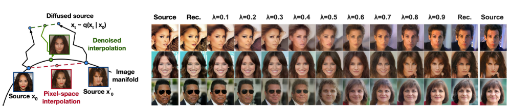
Source image인 $\text{x}_0,\ \text{x}_0'\sim q(\text{x}_0)$를 sampling했을 때, $q$를 stochastic encoder로써 interpolation이 가능하고 reverse process에서 $\text{x}_t,\ \text{x}_t'\sim(\text{x}_t|\text{x}_0)$일 때, linear interpolation을 통해 $\bar{\text{x}}_t=(1-\lambda)\text{x}_0+\lambda\text{x}_0'$를 얻는다. 또한 $\lambda$를 다르게 했을 때, 각각의 source에 가까워지게 reconstruction 되는 것을 확인 할 수 있다.

5. Related Work

Diffusion models는 다른 models와 유사할 수 있지만 $q$의 parameters가 없고 $\text{x}_T$와 $\text{x}_0$간의 mutual information이 zero에 가깝다. Reverse process의 $\epsilon$-prediction은 diffusion models와 denoising score matching 사이에 connection을 만들었다. 그러나 diffusion models는 간단한 log likelihood evaluation을 허용하고 variational inference를 사용하여 Lagevin dynamics sampler를 학습한다. Connection은 또한 denoising score matching의 특정 weighted form이 Langevin과 같은 sampler를 학습하기 위한 variational inference와 동일하다는 의미를 갖는다.

Markov chains의 transition operators를 학습하는 다른 방법은 infusion training, variational walkback, generative stochastic networks 등이 있다.

Score matching과 energy-based modeling에 의해 다른 최근의 연구들에 영향을 줄 수도 있다. 본 논문의 rate-distortion curves는 variational bound의 evaluation에서 시간이 지남에 따라 계산이 되며 annelaed 된 중요도 sampling에서 distortion penalyties에 대해 rate-distortion curves를 계산할 수 있는 방법을 연상시킨다. 본 논문의 progressive decoding은 convolutional DRAW 및 관련 models에서 확인할 수 있으며 autoregressive models의 sampling 전략에 대한 일반적인 설계로 이끌 수 있다.

6. Conclusion

본 논문은 diffusion models를 사용하여 hight quality image samples를 제안했으며 Markov chain의 학습, denoising score matching, annealed Langevin dynmaics, autoregressive models, progressive lossy compression을 위한 diffusion models와 variational inference간의 connection을 발견했다. Diffusion models는 image data에 대한 우수한 inductive biases를 갖고 있는 것으로 보이기 때문에 다른 data modalities와 다른 type의 generative models와 machine learning systems의 구성 요소로써 유용성이 조사가 되기를 기대한다.