아래는 약 1년( 2015년 7월 ~ 2017년 8월 ) 의 기간 동안 수집한 A호텔의 고객 호텔 예약 데이터를 통해 노쇼/취소 고객의 증가를 막고 운영 비용을 노쇼와 취소고객을 예측한 결과에 맞춰 조정하기위해 RandomForestClassifier 모델을 사용한 머신러닝 예측 모델 프로젝트이다.
문제 상황은 이렇다:
🏨🔖
A호텔은 요즘 코로나 여파로 인하여 고생을 겪고 있다. 객실 예약 건수도 줄고 있는 마당에
노쇼/취소 고객도 증가있는 것이 가장 큰 문제이다.
캔슬 고객은 그나마 다행이지만 노쇼 고객의 경우 객실을 하루 날려버리는 것과 같아서, 비용적인 문제에서도 큰 영향을 끼치고 있다.
따라서 노쇼와 취소고객을 사전 예측하고, 운영 비용을 상황에 맞춰 조정하려고 한다.
⛳ 문제정의
▶ 노쇼/취소 고객 증가로 인한 영업이익 감소
⛳ 기대효과
▶ 노쇼/취소 고객 손실 비용 절감, 영업이익 증가
⛳ 해결방안
▶ 노쇼/취소 고객 예측 모델로 고객을 예측하고, 운영 비용 조정
⛳ 성과측정
▶ 모델 활용 노쇼/취소 고객 관리 전/후 손실비용 비교
⛳ 운영
▶ Model에 Input하기 위한 Data mart 생성
▶ 예측 모델 활용 노쇼/취소 고객 추출
▶ 노쇼/취소 가능성이 높은 객실에 대해서는 다른 예약손님을 대체할 수 있도록 준비
데이터셋 정의
# ▶ Data read
import pandas as pd
df = pd.read_csv('S_PJT13_DATA.csv')
df.head()- 컬럼 정보
# hotel: 호텔명 - 호텔의 이름을 나타낸다.
# is_canceled: 취소여부 - 예약이 취소되었는지 여부를 나타낸다. (0: 취소되지 않음, 1: 취소됨)
# lead_time: 입실까지 남은일 - 예약 시점부터 체크인까지 남은 일수를 나타낸다.
# arrival_date_year: 년 - 예약된 체크인 년도를 나타낸다.
# arrival_date_month: 월 - 예약된 체크인 월을 나타낸다.
# arrival_date_week_number: 주 - 예약된 체크인 주 번호를 나타낸다.
# arrival_date_day_of_month: 일 - 예약된 체크인 일을 나타낸다.
# stays_in_weekend_nights: 주말여부 - 투숙 기간 중 주말(금요일 및 토요일) 밤의 수를 나타낸다.
# stays_in_week_nights: 평일여부 - 투숙 기간 중 평일(일요일 ~ 목요일) 밤의 수를 나타낸다.
# adults: 성인 - 예약된 성인 수를 나타낸다.
# children: 어린이 - 예약된 어린이 수를 나타낸다.
# babies: 영유아 - 예약된 영유아 수를 나타낸다.
# meal: 식사 - 예약된 식사 옵션을 나타낸다.
# country: 나라 - 예약자의 국적을 나타낸다.
# market_segment: 예약유통채널상세 - 예약이 유입된 세부 채널을 나타낸다.
# distribution_channel: 예약유통채널 - 예약이 유입된 유통 채널을 나타낸다.
# is_repeated_guest: 기존고객여부 - 재방문 고객인지 여부를 나타낸다. (0: 신규 고객, 1: 재방문 고객)
# previous_cancellations: 과거 취소한 예약수 - 과거에 취소된 예약 횟수를 나타낸다.
# previous_bookings_not_canceled: 과거 취소하지않은 예약수 - 과거에 취소되지 않은 예약 횟수를 나타낸다.
# reserved_room_type: 예약객실타입 - 예약 시 지정된 객실 타입을 나타낸다.
# assigned_room_type: 배정된객실타입 - 실제 배정된 객실 타입을 나타낸다.
# booking_changes: 예약변경횟수 - 예약 후 변경된 횟수를 나타낸다.
# deposit_type: 보증금여부 - 보증금 정책을 나타낸다.
# agent: 여행사ID - 예약을 대행한 여행사의 ID를 나타낸다.
# company: 예약지불회사 - 예약 지불을 처리한 회사의 ID를 나타낸다.
# days_in_waiting_list: 대기자 명단에 있었던 일수 - 대기자 명단에 있었던 기간을 나타낸다.
# customer_type: 계약타입 - 고객의 계약 유형을 나타낸다.
# adr: 평균객실비용 - 평균 일일 객실 요금을 나타낸다.
# required_car_parking_spaces: 요구주차대수 - 요구된 주차 공간의 수를 나타낸다.
# total_of_special_requests: 특별요청수 - 고객이 요청한 특별 요청의 수를 나타낸다.
# reservation_status: 예약상태 - 예약의 현재 상태를 나타낸다. (예: 예약 완료, 체크인, 체크아웃, 취소)
# reservation_status_date: 예약상태 업데이트 날짜 - 예약 상태가 마지막으로 업데이트된 날짜를 나타낸다.
데이터 전처리 및 EDA
(1) Data shape(형태) 확인
# ▶ Data 형태 확인
# ▶ 119,390 row, 32 col로 구성됨
print('df', df.shape)

> df (119390, 32)- 119390 개의 데이터가 있으며 32개의 컬럼으로 이루어져 있음.
(2) Data type 확인
# ▶ Data type 확인
df.info()

<class 'pandas.core.frame.DataFrame'>
<class 'pandas.core.frame.DataFrame'>
RangeIndex: 119390 entries, 0 to 119389
Data columns (total 32 columns):
 #   Column                          Non-Null Count   Dtype
---  ------                          --------------   -----
 0   hotel                           119390 non-null  object
 1   is_canceled                     119390 non-null  int64
 2   lead_time                       119390 non-null  int64
 3   arrival_date_year               119390 non-null  int64
 4   arrival_date_month              119390 non-null  object
 5   arrival_date_week_number        119390 non-null  int64
 6   arrival_date_day_of_month       119390 non-null  int64
 7   stays_in_weekend_nights         119390 non-null  int64
 8   stays_in_week_nights            119390 non-null  int64
 9   adults                          119390 non-null  int64
 10  children                        119386 non-null  float64
 11  babies                          119390 non-null  int64
 12  meal                            119390 non-null  object
 13  country                         118902 non-null  object
 14  market_segment                  119390 non-null  object
 15  distribution_channel            119390 non-null  object
 16  is_repeated_guest               119390 non-null  int64
 17  previous_cancellations          119390 non-null  int64
 18  previous_bookings_not_canceled  119390 non-null  int64
 19  reserved_room_type              119390 non-null  object
 20  assigned_room_type              119390 non-null  object
 21  booking_changes                 119390 non-null  int64
 22  deposit_type                    119390 non-null  object
 23  agent                           103050 non-null  float64
 24  company                         6797 non-null    float64
 25  days_in_waiting_list            119390 non-null  int64
 26  customer_type                   119390 non-null  object
 27  adr                             119390 non-null  float64
 28  required_car_parking_spaces     119390 non-null  int64
 29  total_of_special_requests       119390 non-null  int64
 30  reservation_status              119390 non-null  object
 31  reservation_status_date         119390 non-null  object
dtypes: float64(4), int64(16), object(12)
memory usage: 29.1+ MB
총 31개의 열 데이터가 있으며 노쇼/취소를 할 만한 고객을 선별할 수 있는 의미있는 데이터는 previous_cancellations, is_canceled, is_repeated_guest 등이 있겠다.
그리고 이 중 날짜 데이터인 reservation_status_date 가 object 타입으로 선언되어 있는데 필요에 따라 데이터 분석 진행 시 date 타입으로 변경시키는게 좋을 거 같다.
(3) Null값 확인 (※ 빈 값의 Data)
hotel                                  0
is_canceled                            0
lead_time                              0
arrival_date_year                      0
arrival_date_month                     0
arrival_date_week_number               0
arrival_date_day_of_month              0
stays_in_weekend_nights                0
stays_in_week_nights                   0
adults                                 0
children                               4
babies                                 0
meal                                   0
country                              488
market_segment                         0
distribution_channel                   0
is_repeated_guest                      0
previous_cancellations                 0
previous_bookings_not_canceled         0
reserved_room_type                     0
assigned_room_type                     0
booking_changes                        0
deposit_type                           0
agent                              16340
company                           112593
days_in_waiting_list                   0
customer_type                          0
adr                                    0
required_car_parking_spaces            0
total_of_special_requests              0
reservation_status                     0
reservation_status_date                0
dtype: int64- 일부 열
company와agent등의 값들에 null이 존재한다. null값이 존재할 때 데이터를 처리하기 위해 가장 좋은 방법은 데이터를 완전히 삭제하는 것이 아닌 최대한 보존하는 방향이 좋다.- 따라서 정수형 데이터는 0이나 문자형 데이터는
none과 같은 텍스트로 채워넣는 것이 좋다.
null 값 처리
# ▶ 0 이나 None으로 해석될 수 있는 것은 Drop 하지 않고 채워 넣는다.
df['children'].fillna(0, inplace=True)
df['country'].fillna('none', inplace=True)
df['agent'].fillna(0, inplace=True)
df['company'].fillna(0, inplace=True)
(4) Outlier 확인 (이상치, 정상적인 범주를 벗어난 Data)
# ▶ Outlier 확인
df.describe()
describe()을 통해 전체 통계량을 확인해봤을 때ard즉 평균 일일 객실 요금을 나타내는 평균객실비용의 최소값min값이 음수값으로 분포되어 있어 해당 값을 제거해주어야 한다.
음수값 제거
# ▶ 음수값 제거
df=df[df['adr']>0]
(5) 데이터 EDA
객실 수요 파악
# ▶ 년도별 객실 예약 현황
df['arrival_date_year'].value_counts()

> arrival_date_year
2016    55789
2017    40231
2015    21410
Name: count, dtype: int64
2015년부터 2016년까지는 고객 예약이 급격하게 상승했다가 2017년부터 고객 예약 건수가 줄어든 것을 확인할 수 있다.
# ▶ 월별 객실 예약 현황
df['arrival_date_month'].value_counts()

arrival_date_month
August       13711
July         12491
May          11611
April        10953
October      10929
June         10819
September    10351
March         9641
February      7921
November      6641
December      6561
January       5801
Name: count, dtype: int64
휴가 시즌인 A호텔은 겨울에는 고객 예약수요가 적고 4월을 시작으로 점점 예약 수요가 많아지다 8월 여름 휴가 시즌부터 고객의 객실 예약 수요가 늘어나는 것을 확인할 수 있다.
년, 월별 객실 이용 현황
# ▶ 년, 월별 객실 이용 현황 확인
df_reservation = pd.DataFrame(df.groupby(['arrival_date_year', 'arrival_date_month'], as_index=False)['hotel'].count())
df_reservation.head(10)

	arrival_date_year	arrival_date_month	hotel
0				 2015				August	 3794
1				 2015			  December	 2795
2				 2015				  July	 2714
3				 2015			  November	 2274
4				 2015			   October	 4824
5				 2015			 September	 5009
6				 2016				 April	 5346
7				 2016				August	 5020
8				 2016			  December	 3766
9				 2016			  February	 3820
해당 월 데이터가 문자열로 되어 있어 어떤 달인지 확실히 식별이 어려워서 월 데이터를 재정의
해주었다.
# ▶ replace 함수를 활용하여 월 데이터 재정의
df_reservation = df_reservation.replace({'January' : '01.January',
                                         'February' : '02.February',
                                         'March' : '03.March',
                                         'April' : '04.April',
                                         'May' : '05.May',
                                         'June' : '06.June',
                                         'July' : '07.July',
                                         'August' : '08.August',
                                         'September' : '09.September',
                                         'October' : '10.October',
                                         'November' : '11.November',
                                         'December' : '12.December'})
df_reservation.head(5)

	arrival_date_year	arrival_date_month	hotel
0				 2015			 08.August	 3794
1				 2015		   12.December	 2795
2				 2015			   07.July	 2714
3		 		 2015		   11.November	 2274
4				 2015		    10.October	 4824
훨씬 보기 깔끔해짐. 이후 년, 월별 객실 이용 현황을 전체적으로 출력해보았다.
# ▶ Plotting하기 어려움
df_reservation = df_reservation.sort_values(by=['arrival_date_year','arrival_date_month'])
df_reservation

	arrival_date_year	arrival_date_month	hotel
2				 2015		       07.July	2714
0				 2015			 08.August	3794
5				 2015		   09.September	5009
4				 2015			 10.October	4824
3				 2015		    11.November	2274
1				 2015			12.December	2795
10				 2016			 01.January	2183
9				 2016			02.February	3820
13				 2016	 		   03.March	4739
6				 2016			   04.April	5346
14	 			 2016				 05.May	5367
12				 2016				06.June	5227
11				 2016				07.July	4507
7				 2016			  08.August	5020
17				 2016		   09.September	5342
16				 2016			 10.October	6105
15				 2016			11.November	4367
8				 2016			12.December	3766
21				 2017			 01.January	3618
20				 2017			02.February	4101
24				 2017			   03.March	4902
18				 2017			   04.April	5607
25				 2017				 05.May	6244
23				 2017				06.June	5592
22				 2017				07.July	5270
19				 2017			  08.August	4897
- 년, 월별 객실 이용 현황을 년도별로
Sorting하여 내림차순 한 결과, 2015년은 7월부터 데이터 존재, 2016년은 12개월 모두 존재, 2017년은 1~8월까지만 존재하는 것을 확인할 수 있다. - 하지만 각 년, 월별로 이용 현황이 어떠한지 데이터가 너무 많아 분포를 확인하기가 어려워 시각화를 하였다.
# ▶ barplot, order 옵션을 활용하여 가독성 Up
import matplotlib.pyplot as plt
import seaborn as sns
%matplotlib inline
plt.style.use(['dark_background'])

sns.barplot(x='arrival_date_month', y='hotel', hue='arrival_date_year', data = df_reservation,
            order = ['01.January', '02.February', '03.March', '04.April', '05.May', '06.June', '07.July', '08.August', '09.September', '10.October', '11.November', '12.December']);
plt.gcf().set_size_inches(20, 5);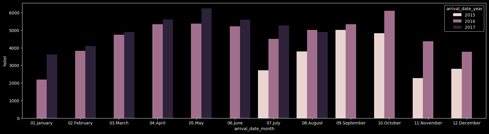
-
데이터를 확인해보니 모든 데이터가 5월~8월 사이에 예약 수요가 가장 많이 급증한 것을 알 수 있으며 공통적으로 겨울
novermber,december에 고객 에약 수요가 줄어든 것을 확인할 수 가 있다.
취소고객, 노쇼 고객 특성 분석
이제 전체적인 데이터 EDA를 완료했으니 A호텔의 영업이익을 감소시키는 원인인 노쇼 고객 또는 예약 취소 고객을 분석해보겠다.
(1) 취소 및 노쇼 비율
일단 'reservation_status' 즉 전체적인 예약의 현황을 살펴보았다.
df['reservation_status'].value_counts()

reservation_status
Check-Out    73419
Canceled     42830
No-Show       1181
예약 현황을 확인해보니 check_out 건을 제외하고 취소건은 42830 건, 예약은 했지만 노쇼한 건 수가 1181개나 되는 것을 확인했다.
이렇게 숫자로 나타난 예약 현황들을 활용해 전체 예약 취소 건의 비율과 노쇼 건의 비율을 계산해 볼 수 있겠다.
# ▶ 캔슬 비율
print('Canceled :', 42830 / (73419 + 42830 + 1181))


# ▶ 노쇼 비율
print('No-Show :', 1181 / (73419 + 42830 + 1181))

>Canceled : 0.36472792301796814
>No-Show : 0.010057055266967554- 확인을 해보니 취소 건수는 전체 예약 건수의 36프로나 차지하고 있었다.
- 노쇼의 비율은 전체 예약 건수에서 1프로 정도만 차지 하고 있다.
- 그래서 취소 건수와 노쇼 건을 따로 나눠서 예측하는 것보다 취소와 노쇼 건을 하나로 묶어서 예측 모델링을 만들기 위해 checkout 된 건수는 0으로 취소와 노쇼에 대한 건수는 1로 변경하기로 한다.
# ▶ checkout된 예약 건수는 0으로 취소 노쇼에 대한 데이터는 1로 변경
import numpy as np
df['reservation_status'] = np.where(df['reservation_status'] != 'Check-Out', 1, 0)
df['reservation_status'].value_counts()

reservation_status
0    73419
1    44011
Name: count, dtype: int64
(2) 취소 및 노쇼 고객 특성 분석
데이터 시각화를 통해 정상적으로 checkout된 건수와 취소 및 노쇼 건수의 월 별 분포를 확인해보았다.
A호텔 월 별 예약 현황 분포
# ▶ 월에 따른 취소/노쇼율 비교
sns.catplot(x="arrival_date_month", hue="reservation_status", kind="count",palette="pastel", edgecolor=".6",data=df,
            order = ['January', 'February', 'March', 'April', 'May', 'June', 'July', 'August', 'September', 'October', 'November', 'December']);
plt.gcf().set_size_inches(20, 3)
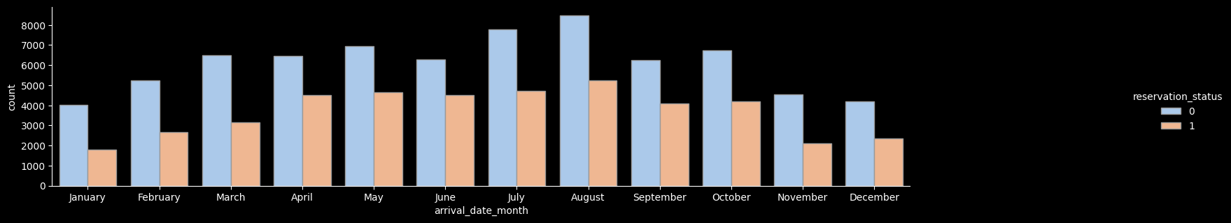
- 육안으로 그래프 확인 결과 가장 많은 예약취소나 노쇼가 있는 달은
August8월 달에 예약 건수가 가장 많은 만큼 예약취소나 노쇼가 많은 것을 확인할 수 있다. - 정확한 월 별 취소/노쇼가 가장 많은 달이 어떤 것인지 확인하기 위해서는 취소/노쇼의 분포만 보는 것이 아닌 예약 건수에 따라 월 별로 취소/노쇼의 비율을 데이터 프레임화 해보았다.
# ▶ 월에 따른 취소/노쇼율 비교
df_gp = df.groupby('arrival_date_month')['reservation_status'].agg(['count','sum'])
df_gp.head()

df_gp['ratio'] = round((df_gp['sum'] / df_gp['count']) * 100, 1)
df_gp = df_gp.sort_values(by=['ratio'], ascending=False)
df_gp

   				   count   sum  ratio
arrival_date_month
June               10819  4523   41.8
April              10953  4504   41.1
May                11611  4659   40.1
September          10351  4092   39.5
October            10929  4209   38.5
August             13711  5228   38.1
July               12491  4723   37.8
December            6561  2355   35.9
February            7921  2676   33.8
March               9641  3137   32.5
November            6641  2110   31.8
January 5801 1795 30.9- 육안으로 그래프를 봤을 때는 8월 달이 가장 예약/취소 건수가 많았지만 실제 예약 건수에 따른 노쇼/취소 건수의 비율을 확인해보니 6월달, 4월달, 5월달이 예약 취소/노쇼가 가장 많은 것을 확인할 수 있다.
A호텔 호텔 타입에 따른 취소/노쇼 예약 분포 및 비율
# ▶ Resort Hotel과 City Hotel 비교
sns.catplot(x="hotel", hue="reservation_status", kind="count",palette="pastel", edgecolor=".6",data=df);
plt.gcf().set_size_inches(20, 3)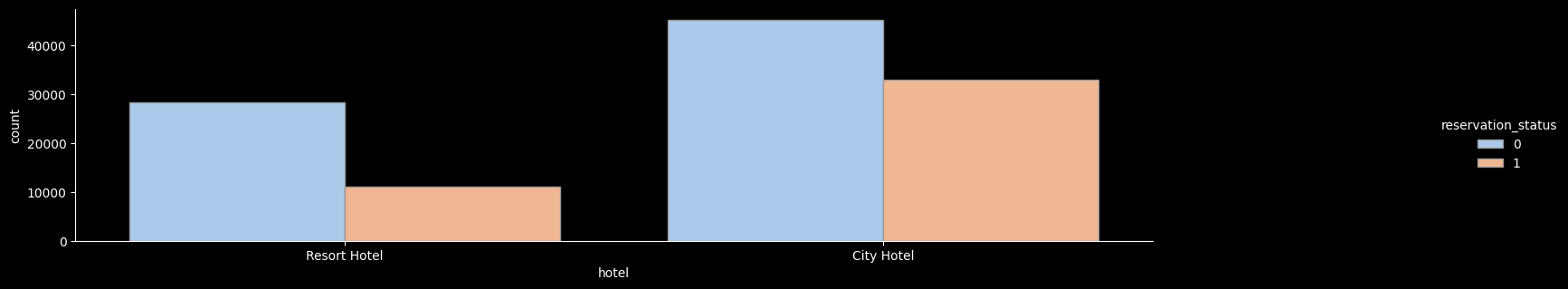
호텔의 타입에 따른 예약 checkout 그리고 취소/노쇼 건수의 분포를 확인해보니 city hotel의 예약 취소/노쇼의 분포가 가장 많은 것을 확인할 수 있었다.
정확한 취소/노쇼의 비율을 데이터프레임화 해서 확인해 보았다.
# ▶ Resort Hotle과 City Hotel 비교
df_gp = df.groupby('hotel')['reservation_status'].agg(['count','sum'])
df_gp['ratio'] = round((df_gp['sum'] / df_gp['count']) * 100, 1)
df_gp = df_gp.sort_values(by=['ratio'], ascending=False)
df_gp

				   count   sum  ratio
			hotel
City Hotel		   78122 32973	 42.2
Resort Hotel	   39308 11038	 28.1
마찬가지로 호텔의 타입에 따른 예약 checkout 그리고 취소/노쇼 건수의 비율을 확인해보니
city hotel의 예약 취소/노쇼의 분포가 압도적으로 극단적으로 많은 것을 확인할 수 있었다.
그래서 city hotel의 예약 취소/노쇼의 원인을 파악하거나 운영을 관리가 필요할 것으로 보인다.
A호텔 주말 예약 일수에 따른 노쇼/취소 고객 비교
# ▶ 주말 예약 일수에 따른 비교
sns.catplot(x="stays_in_weekend_nights", hue="reservation_status", kind="count",palette="pastel", edgecolor=".6",data=df);
plt.gcf().set_size_inches(20, 3)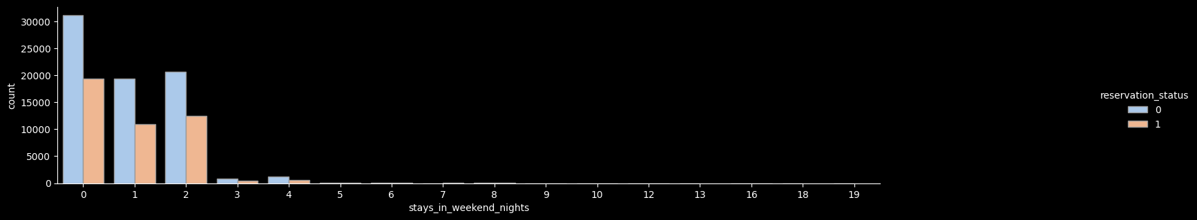
호텔의 주말 예약 일수에 따른 분포를 비교해본 결과 거의 0~2일의 주말이 예약 일수에 끼어있는 예약이 많이 분포되어 있고 3일, 4일, 6일, 9일 등 주말 예약 일수가 많은 예약도 일부 존재하는 것을 확인할 수 있었다.
주말 예약 일수에 따른 정확한 취소/노쇼의 비율을 데이터프레임화 해서 확인해 보았다.
# ▶ 주말 예약 일수에 따른 비교
df_gp = df.groupby('stays_in_weekend_nights')['reservation_status'].agg(['count','sum'])
df_gp['ratio'] = round((df_gp['sum'] / df_gp['count']) * 100, 1)
df_gp = df_gp.sort_values(by=['ratio'], ascending=False)
df_gp

				   		count   sum  ratio
stays_in_weekend_nights
		9					9	  7	  77.8
		7				   19	 14	  73.7
		8				   57	 34	  59.6
		6				  152	 87	  57.2
		5				   77	 43	  55.8
		0				50499  19361  38.3
		2				33150  12453  37.6
		1				30361  10967  36.1
		3				 1244	 444  35.7
	   16					3	   1  33.3
	    4				 1844	 597  32.4
	   10					7	   2  28.6
	   12					5	   1  20.0
	   13					1	   0   0.0
	   18					1	   0   0.0
	   19					1	   0   0.0
주말 예약 일수에 따른 취소/노쇼 비율을 확인해보니 9일 8일 8일 6일 등 주말 에약 일수가 많을 수록 취소/노쇼를 하는 고객의 비율이 많은 것을 확인할 수 있었다.
그리고 주말 예약 일수가 0~2일이 있는 예약 건의 취소/노쇼 비율이 큰 차이가 없는 것으로 보아 주말이 없어 0인 평일에 예약한 건수들과 주말에 1~2일 예약한 건수들의 비율이 큰 차이가 없어 유의미한 데이터라고 보기가 어려울 거 같다.
그래서 더 넓은 분포 및 비율을 보기 위해 주말 예약 일수가 2일 이하인 것은 1, 8일 이하인 것은 2, 그 이외에는 3으로 그룹핑하여 구간화로 주말 일수별 예약 취소/노쇼 비율을 비교했다.
# ▶ 주말 예약 일수에 따른 비교(re-binning)
df_c = df.copy()

df_c['gp'] = np.where(df_c['stays_in_weekend_nights'] <= 2, 1,
                      np.where(df_c['stays_in_weekend_nights'] <= 8, 2, 3))

df_gp = df_c.groupby('gp')['reservation_status'].agg(['count','sum'])
df_gp['ratio'] = round((df_gp['sum'] / df_gp['count']) * 100, 1)
df_gp = df_gp.sort_values(by=['ratio'], ascending=False)
df_gp


>
    count    sum  ratio
gp
3      27     11   40.7
1  114010  42781   37.5
2 3393 1219 35.9- 예약 취소/노쇼가 가장 많은 것은 주말 예약 일수가 9일 이상인 경우가 가장 많은 취소 비율을 보였고 그 다음으로 2일 이하인 경우 그리고 8일 이하인 경우가 가장 많이 차지했다.
- 하지만 9일 이상인 경우의 데이터의 수가 너무 작아서 27명의 데이터를 가지고만 주말 일수가 많음에 따라 취소/노쇼 비율이 높다라고 추정을 하기는 어렵겠다.
A호텔 객실 타입에 따른 예약 일수/ 취소 및 노쇼 비율
# ▶ 객실타입에 따른 비교
df_gp = df.groupby('reserved_room_type')['reservation_status'].agg(['count','sum'])
df_gp['ratio'] = round((df_gp['sum'] / df_gp['count']) * 100, 1)
df_gp = df_gp.sort_values(by=['ratio'], ascending=False)
df_gp

                    count    sum  ratio
reserved_room_type
H                    595    245   41.2
A                  84573  33477   39.6
G                   2006    756   37.7
B                   1085    365   33.6
C                    913    306   33.5
L                      6      2   33.3
D                  19005   6086   32.0
F                   2824    873   30.9
E                   6423   1901   29.6
객실 타입에 따른 예약 취소/노쇼 비율을 확인해보니 H 룸타입과 A룸타입의 취소/노쇼 비율이 가장 높았다.
A호텔의 lead time, 즉 예약일로부터 checkout 날까지 남은 기간에 따른 노쇼/취소 비율
# ▶ lead time
sns.distplot(df['lead_time']); 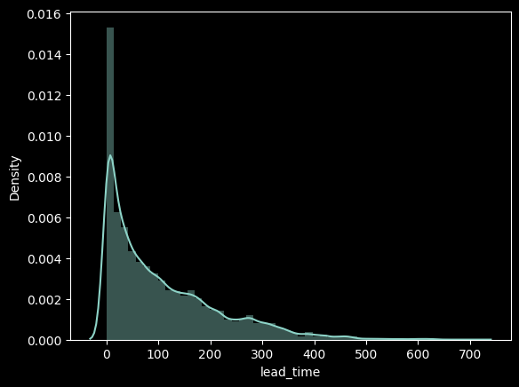
예약일로부터 checkout 날까지 남은 기간에 따른 노쇼/취소 고객의 분포를 확인해보니 비교적 예약일이 얼마 안남은 시점 순으로부터 노쇼/취소고객이 많은 것을 확인할 수 있었고 정확한 비율 확인을 위해 입실일로부터 100일이하가 남은 예약을 1, 200일 이하가 남은 예약을 2, 나머지 200일이 초과하는 예약을 3으로 지정하고 다시 비율을 만들어보았다.
# ▶ lead time 구간화
df_c = df.copy()
df_c['gp'] = np.where(df['lead_time'] <= 100, 1,
                       np.where(df['lead_time']<=200, 2, 3))

df_gp = df_c.groupby('gp')['reservation_status'].agg(['count','sum'])
df_gp['ratio'] = round((df_gp['sum'] / df_gp['count']) * 100, 1)
df_gp = df_gp.sort_values(by=['ratio'], ascending=False)
df_gp

	count	  sum	ratio
gp
3	20526	12182	 59.3
2	26586	11987	 45.1
1 70318 19842 28.2- 확인 결과 예약 건수에 비해서 입실일이 200일이 넘게 남은 고객들의 취소 비율이 가장 높았고 그 뒤로 200일 이하, 100일 이하 순으로 고객의 취소 비율이 이어졌다.
결론
-
확인 결과 예약 건수에 비해서 입실일이 200일이 넘게 남은 고객들의 취소 비율이 가장 높았고 그 뒤로 200일 이하, 100일 이하 순으로 고객의 취소 비율이 이어졌다.
-
마찬가지로 호텔의 타입에 따른 예약 checkout 그리고 취소/노쇼 건수의 비율을 확인해보니
city hotel의 예약 취소/노쇼의 분포가 압도적으로 극단적으로 많은 것을 확인할 수 있었다.
그래서city hotel의 예약 취소/노쇼의 원인을 파악하거나 운영을 관리가 필요할 것으로 보인다.- 육안으로 그래프를 봤을 때는 8월 달이 가장 예약/취소 건수가 많았지만 실제 예약 건수에 따른 노쇼/취소 건수의 비율을 확인해보니 6월달, 4월달, 5월달이 예약 취소/노쇼가 가장 많은 것을 확인할 수 있다.