아래는 A 영화 회사의 신규 영화 촬영 시기가 다가오고 제작비를 효율적으로 관리하고 수익을 최대화하고 싶어한다. 매출을 극대화할 수 있는 성우를 찾기위해 영화의 순위와 영화에 캐스팅된 성우들에 대한 분석을 진행한 프로젝트이다.
여러 개의 csv 파일로 분석을 진행하는 복잡한 프로젝트이다.
문제 상황은 이렇다:
🔖
A사는 이번에 신규 영화를 촬영할 계획을 가지고 있다. 제작비가 크게 들어가는 만큼 그 만큼의 수익이 발생해야하는 상황이기 때문에 최대한 Risk를 덜 가져가려고 하고 있다. 이에 과거 상영한 영화의 데이터를 활용하여 감독, 성우에 따라 매출을 극대화하는 캐스팅을 진행하려고 한다.
⛳ 문제정의
▶ 신규 영화 제작을 위한 캐스팅 Line-up 불분명
⛳ 기대효과
▶ 매출을 극대화 할 수 있는 감독 및 배우 캐스팅 및 영화 흥행
⛳ 해결방안
▶ 과거 영화 데이터 활용 매출 극대화 캐스팅
⛳ 성과측정
▶ 캐스팅 후 영화 제작 및 상영 후 매출 모니터링
⛳ 운영
▶ 캐스팅 결과 활용
데이터셋 정의
# ▶ Movie total gross
import pandas as pd
df_movie_gross = pd.read_csv('S_PJT14_disney_movies_total_gross.csv')

print(df_movie_gross.shape)
df_movie_gross.head()

   index                     movie_title  release_date     	genre 	MPAA_rating     total_gross inflation_adjusted_gross
0      0  Snow White and the Seven Dwarfs  Dec 21, 1937    Musical            G   $184,925,485            $5,228,953,251
1      1                        Pinocchio   Feb 9, 1940  Adventure            G    $84,300,000             $2,188,229,052
2      2                         Fantasia  Nov 13, 1940    Musical            G    $83,320,000             $2,187,090,808
3      3                Song of the South  Nov 12, 1946  Adventure            G    $65,000,000             $1,078,510,579
4      4                       Cinderella  Feb 15, 1950      Drama            G    $85,000,000               $920,608,730
| index | movie_title | release_date | genre | MPAA_rating | total_gross | inflation_adjusted_gross |
|---|---|---|---|---|---|---|
| 인덱스 | 영화제목 | 출시일 | 장르 | 영화시청등급 | 해당 영화 총 수익 | 인플레이션 대비 수익 |
데이터 전처리 및 EDA
(1) movie_gross Data shape(형태) 확인
# ▶ Data 형태 확인
# ▶ 7,043 row, 21 col로 구성됨
df_movie_gross.shape

> (579, 7)- 영화의 매출 및 수익 데이터는 579개의 행과 7개의 열 데이터가 있다.
(2) movie_gross Data type 확인
# ▶ Data type 확인
df.info()

<class 'pandas.core.frame.DataFrame'>
RangeIndex: 579 entries, 0 to 578
Data columns (total 7 columns):
 #   Column                    Non-Null Count  Dtype
---  ------                    --------------  -----
 0   index                     579 non-null    int64
 1   movie_title               579 non-null    object
 2   release_date              579 non-null    object
 3   genre                     562 non-null    object
 4   MPAA_rating               523 non-null    object
 5   total_gross               579 non-null    object
 6   inflation_adjusted_gross  579 non-null    object
dtypes: int64(1), object(6)
memory usage: 31.8+ KB
총 21개의 열 데이터가 있으며 total_gross, inflation_adjusted_gross 라는 돈의 데이터가 있는 값들이 숫자형 데이터가 아닌 object 문자형 데이터로 선언이 돼있다.
그리고 release_date와 같이 날짜형 데이터 타입이어야 할 데이터가 object 문자형 데이터로 선언이 되어있다.
필요에 따라 데이터 분석 진행 시 int 타입 그리고 날짜형 데이터는 date 타입으로 변경시키는게 좋을 거 같다.
(3) movie_gross Null값 확인 (※ 빈 값의 Data)
df_movie_gross.isnull().sum()

index                        0
movie_title                  0
release_date                 0
genre                       17
MPAA_rating                 56
total_gross                  0
inflation_adjusted_gross     0
dtype: int64null값이 존재하며 해당null값들은 제거해주거나 문자열none또는 0 으로 대체해줄 것이다.
문자열 데이터 전처리 및 Null 처리
# ▶ 문자열 데이터 전처리 및 Null 처리
df_movie_gross['inflation_adjusted_gross'] = df_movie_gross['inflation_adjusted_gross'].str.replace('$', '')
df_movie_gross['inflation_adjusted_gross'] = df_movie_gross['inflation_adjusted_gross'].str.replace(',', '')
df_movie_gross['inflation_adjusted_gross'] = df_movie_gross['inflation_adjusted_gross'].str.replace('\r', '')
df_movie_gross['inflation_adjusted_gross'] = df_movie_gross['inflation_adjusted_gross'].astype(int)

df_movie_gross['total_gross'] = df_movie_gross['total_gross'].str.replace('$', '')
df_movie_gross['total_gross'] = df_movie_gross['total_gross'].str.replace(',', '')
df_movie_gross['total_gross'] = df_movie_gross['total_gross'].str.replace('\r', '')
df_movie_gross['total_gross'] = df_movie_gross['total_gross'].astype(int)

df_movie_gross['genre'].fillna('none', inplace = True)
df_movie_gross['MPAA_rating'].fillna('none', inplace = True)

df_movie_gross = df_movie_gross.drop(['index'], axis=1)
df_movie_gross.head(5)df_movie_gross.info()
<class 'pandas.core.frame.DataFrame'>
RangeIndex: 579 entries, 0 to 578
Data columns (total 6 columns):
# Column Non-Null Count Dtype
--- ------ -------------- -----
0 movie_title 579 non-null object
1 release_date 579 non-null object
2 genre 579 non-null object
3 MPAA_rating 579 non-null object
4 total_gross 579 non-null int64
5 inflation_adjusted_gross 579 non-null int64
dtypes: int64(2), object(4)
memory usage: 27.3+ KB문자열 데이터 타입이었던 데이터들을 int64 숫자형으로 변형시켜주었다.
# ▶ 시간 데이터 변환
df_movie_gross['release_date'] = pd.to_datetime(df_movie_gross['release_date'])
df.info()

<class 'pandas.core.frame.DataFrame'>
RangeIndex: 579 entries, 0 to 578
Data columns (total 6 columns):
 #   Column                    Non-Null Count  Dtype
---  ------                    --------------  -----
 0   movie_title               579 non-null    object
 1   release_date              579 non-null    datetime64[ns]
 2   genre                     579 non-null    object
 3   MPAA_rating               579 non-null    object
 4   total_gross               579 non-null    int64
 5   inflation_adjusted_gross  579 non-null    int64
dtypes: datetime64[ns](1), int64(2), object(3)
memory usage: 27.3+ KB
release_date 도 날짜형 데이터 타입으로 변형해주었다.
(4) movie_gross 데이터 중복 데이터 확인
# ▶ 영화별 중복 데이터 존재
df_movie_gross['movie_title'].value_counts()

The Jungle Book                 3
Freaky Friday                   2
Cinderella                      2
Bad Company                     2
101 Dalmatians                  2
                               ..
Quiz Show                       1
A Simple Twist of Fate          1
It's Pat                        1
Camp Nowhere                    1
Rogue One: A Star Wars Story    1
Name: movie_title, Length: 573, dtype: int64- 확인 결과 일부 영화들이 중복된 데이터가 있는 것으로 보인다.
# ▶ 정글북이여도, 장르와 발매년도에 따라 여러개의 데이터가 존재
df_movie_gross[df_movie_gross['movie_title'] == 'The Jungle Book']

				     movie_title  release_date	    genre	MPAA_rating		total_gross	inflation_adjusted_gross
13				 The Jungle Book	1967-10-18	  Musical	  Not Rated		  141843000				   789612346
194				 The Jungle Book	1994-12-25	Adventure			 PG		   44342956					88930321
567 The Jungle Book 2016-04-15 Adventure PG 364001123 364001123- 구체적으로 예를 들어 같은 정글북 영화여도 장르와 발매년도에 따라 여러개의 데이터가 존재하고 있었다.
# ▶ 같은 영화라면 최신에 개봉한 영화만 남기기
df_movie_gross = df_movie_gross.sort_values(by=['movie_title', 'release_date'], ascending=[True, False])
df_movie_gross = df_movie_gross.drop_duplicates('movie_title', keep='first')
df_movie_gross.head(5)

|       movie_title        | release_date |    genre   | MPAA_rating | total_gross | inflation_adjusted_gross |
|--------------------------|--------------|------------|-------------|-------------|--------------------------|
| 101 Dalmatians           | 1996-11-27   | Comedy     | G           | 136189294   | 258728898                |
| 102 Dalmatians           | 2000-11-22   | Comedy     | G           | 66941559    | 104055039                |
| 1492: Conquest of Paradise| 1992-10-09   | Adventure  | PG-13       | 7099531     | 14421454                 |
| 20,000 Leagues Under the Sea | 1954-12-23 | Adventure  | none        | 28200000    | 528279994                |
| 25th Hour                | 2002-12-19   | Drama      | R           | 13084595    | 18325463                 |
# ▶ 중복제거 확인
df_movie_gross['movie_title'].value_counts().head(5)
101 Dalmatians 1
Stakeout 1
Song of the South 1
Sorority Boys 1
Spaced Invaders 1
Name: movie_title, dtype: int64그래서 중복되는 다른 영화 데이터는 제거하고 가장 최신에 개봉한 영화만 남기도록 하였다.
(1) Voice actor data Data shape(형태) 확인
# ▶ Voice actor
import pandas as pd
df_voice_actor = pd.read_csv('S_PJT14_disney_voice_actors.csv')
print(df_voice_actor.shape)
df_voice_actor.head(5)

> (935, 4)
index	       character	      voice-actor 				  		  movie
0	0	    Abby Mallard  		  Joan Cusack 				 Chicken Little
1	1	  Abigail Gabble		 Monica Evans 		 		 The Aristocats
2	2		    Abis Mal	  Jason Alexander			The Return of Jafar
3	3	Abu						 Frank Welker						Aladdin
4 4 Achilles NaN The Hunchback of Notre Dame- 영화 성우의 데이터는 935개의 행과 4개의 열 데이터가 있다.
# ▶ Col 재정비
df_voice_actor = df_voice_actor[['movie', 'character', 'voice-actor']]
df_voice_actor.columns = ['movie_title', 'character', 'voice_actor']
df_voice_actor.head(5)

					movie_title	character	voice_actor
0				  Chicken Little	Abby Mallard	Joan Cusack
1				  The Aristocats	Abigail Gabble	Monica Evans
2	The Return of Jafar	Abis Mal	Jason Alexander
3	Aladdin	Abu	Frank Welker
4	The Hunchback of Notre Dame	Achilles	None
불필요한 인덱스 컬럼이 존재해 제거해주었다.
(2)Voice actor data Null값 확인 (※ 빈 값의 Data)
df_voice_actor.isnull().sum()

index          0
character      0
voice-actor    0
movie          0
dtype: int64null값이 존재하지 않는다.
(3) Voice actor data 데이터 중복 데이터 확인
# ▶ 하나의 영화에 참여만 여러명의 성우가 존재한다.
df_voice_actor['movie_title'].value_counts()

DuckTales             31
Zootopia              22
Hercules              22
Wreck-It Ralph        21
The Little Mermaid    20
                      ..
The Plow Boy           1
Hold That Pose         1
Grin and Bear It       1
Saludos Amigos         1
The Pirate Fairy       1
Name: movie_title, Length: 139, dtype: int64- 확인 결과 중복 데이터가 있지만 하나의 영화에 참여한 여러명의 성우가 존재하는 것으로 보이며 한 영화의 제목에 여러명의 성우가 존재하는 것이기에 중복이라고 보기 어렵다.
(1) Director data Data shape(형태) 확인
# ▶ Data 형태 확인
# ▶ Movie director
df_director = pd.read_csv('S_PJT14_disney_director.csv')
print(df_director.shape)
df_director.head(5)

> (56, 3)
index							   name		  director
0	0	Snow White and the Seven Dwarfs		David Hand
1	1						  Pinocchio	Ben Sharpsteen
2	2						   Fantasia	  full credits
3	3							  Dumbo	Ben Sharpsteen
4	4							  Bambi		David Hand
- 감독에 대한 데이터는 56개의 행과 3개의 열 데이터가 있다.
df_director = df_director[['name', 'director']]
df_director.columns = ['movie_title', 'director']
df_director.head(5)

							   name		  director
0	Snow White and the Seven Dwarfs		David Hand
1						  Pinocchio	Ben Sharpsteen
2						   Fantasia	  full credits
3							  Dumbo	Ben Sharpsteen
4							  Bambi		David Hand
불필요한 인덱스 컬럼이 존재해 인덱스 컬럼을 제거해주었다.
(2) Director data Null값 확인 (※ 빈 값의 Data)
df_director.isnull().sum()

index       0
name        0
director    0
dtype: int64null값이 존재하지 않는다.
(3) Director data 데이터 중복 데이터 확인
# ▶ 중복없음
df_director['movie_title'].value_counts().head(5)

Snow White and the Seven Dwarfs    1
Pinocchio                          1
Aladdin                            1
The Lion King                      1
Pocahontas                         1
Name: movie_title, dtype: int64- 각각의 영화에서 중복된 감독은 존재하지 않는다.
(1) Song dataData shape(형태) 확인
# ▶ Movie song
df_song = pd.read_csv('S_PJT14_disney_characters.csv')
print(df_song.shape)
df_song.head(5)

> (56, 6)
|   index |            movie_title             |   release_date   |    hero     |   villian   |             song              |
|---------|------------------------------------|------------------|-------------|-------------|-------------------------------|
|       0 | \nSnow White and the Seven Dwarfs    | December 21, 1937| Snow White  | Evil Queen  | Some Day My Prince Will Come  |
|       1 | \nPinocchio                          | February 7, 1940 | Pinocchio   | Stromboli   | When You Wish upon a Star     |
|       2 | \nFantasia                           | November 13, 1940| NaN         | Chernabog   | NaN                           |
|       3 | \nDumbo                              | October 23, 1941 | Dumbo       | Ringmaster  | Baby Mine                     |
|       4 | \nBambi                              | August 13, 1942  | Bambi       | Hunter      | Love Is a Song                |
- 영화에 쓰인 노래 또는 OST에 대한 데이터는 56개의 행과 6개의 열 데이터가 있다.
- 해당 데이터셋의 영화 제목을 보니
\n이라는 문자열이 포함되어 있는 것으로 보아 해당 문자열을 제거해주어야 할 것으로 보인다.
(2) Song data Null값 확인 (※ 빈 값의 Data)
df_song.isnull().sum()

index            0
movie_title      0
release_date     0
hero             4
villian         10
song             9
dtype: int64herovillian열에 일부null값이 존재하는 것으로 보인다.none` 값으로 대체해주어야 할 것으로 보인다.
데이터 전처리
# ▶ 문자열 데이터 처리
import re
df_song['movie_title'] = df_song['movie_title'].str.replace('\n', '')
df_song.fillna('none', inplace=True)
df_song.drop(['index'], axis=1, inplace =True)
df_song.head(5)


|            movie_title             |   release_date   |    hero     |   villian   |             song              |
|------------------------------------|------------------|-------------|-------------|-------------------------------|
| Snow White and the Seven Dwarfs    | December 21, 1937| Snow White  | Evil Queen  | Some Day My Prince Will Come  |
| Pinocchio                          | February 7, 1940 | Pinocchio   | Stromboli   | When You Wish upon a Star     |
| Fantasia                           | November 13, 1940| NaN         | Chernabog   | NaN                           |
| Dumbo                              | October 23, 1941 | Dumbo       | Ringmaster  | Baby Mine                     |
| Bambi                              | August 13, 1942  | Bambi       | Hunter      | Love Is a Song                |
- 앞서 영화 제목에 있던
\n을 제거해주고 불필요한index컬럼을 제거해주었다. null값 데이터는none으로 변경해주었다.
(3) Song data 데이터 중복 데이터 확인
# ▶ 중복 없음
df_song['movie_title'].value_counts().head(5)

Snow White and the Seven Dwarfs    1
Pinocchio                          1
Aladdin                            1
The Lion King                      1
Pocahontas                         1
Name: movie_title, dtype: int64- 각각의 영화에 쓰인 중복된 영화는 존재하지 않는다.
(5) 데이터 EDA
Data 연결
현재 영화 데이터는 총 4개로 쪼개져 있는 상황으로 효율적인 분석을 위해서는 4개의 데이터를 하나로 merge 병합해야 한다. 각각의 데이터의 특징은 이렇다.
- df_movie_gross : 영화 수익 (Base data) - 중복 X
- df_voice_actor : 영화 캐릭터 별 성우 - 중복 O
- df_director : 영화 감독 - 중복 X
- df_song : 영화 OST 및 히어로/빌런 - 중복 X
그래서 중복이 없는 데이터를 우선하여 병합을 해주었다.
# ▶ 중복 없는 데이터 우선 merge
|       movie_title        | release_date |    genre   | MPAA_rating | total_gross | inflation_adjusted_gross |       director        |
|--------------------------|--------------|------------|-------------|-------------|--------------------------|------------------------|
| 101 Dalmatians           | 1996-11-27   | Comedy     | G           | 136189294   | 258728898                | Wolfgang Reitherman    |
| 102 Dalmatians           | 2000-11-22   | Comedy     | G           | 66941559    | 104055039                | NaN                    |
| 1492: Conquest of Paradise| 1992-10-09   | Adventure  | PG-13       | 7099531     | 14421454                 | NaN                    |
| 20,000 Leagues Under the Sea | 1954-12-23 | Adventure  | none        | 28200000    | 528279994                | NaN                    |
| 25th Hour                | 2002-12-19   | Drama      | R           | 13084595    | 18325463                 | NaN                    |


Churn
No     5174
Yes    1869
Name: count, dtype: int64
다음으로 df_song 데이터 프레임을 병합하기 위해 겹치는 데이터인 release_date 열을 제거해주었다.
# ▶ df_song에 release_date 중복 col 이기에 제거 후 merge
df_song = df_song.drop(['release_date'], axis=1)
df_merge = pd.merge(df_merge, df_song, how='left', on='movie_title')
df_merge.head(5)

|       movie_title        | release_date |    genre   | MPAA_rating | total_gross | inflation_adjusted_gross |       director        |  hero | villian | song |
|--------------------------|--------------|------------|-------------|-------------|--------------------------|------------------------|-------|---------|------|
| 101 Dalmatians           | 1996-11-27   | Comedy     | G           | 136189294   | 258728898                | Wolfgang Reitherman    |  NaN  |   NaN   | NaN  |
| 102 Dalmatians           | 2000-11-22   | Comedy     | G           | 66941559    | 104055039                | NaN                    |  NaN  |   NaN   | NaN  |
| 1492: Conquest of Paradise| 1992-10-09   | Adventure  | PG-13       | 7099531     | 14421454                 | NaN                    |  NaN  |   NaN   | NaN  |
| 20,000 Leagues Under the Sea | 1954-12-23 | Adventure  | none        | 28200000    | 528279994                | NaN                    |  NaN  |   NaN   | NaN  |
| 25th Hour                | 2002-12-19   | Drama      | R           | 13084595    | 18325463                 | NaN                    |  NaN  |   NaN   | NaN  |
데이터를 병합해보니 전체적인 null 값이 많은 것으로 보여 각 데이터들의 shape 형태를 확인해보았다.
# ▶ Target 숫자 데이터로 변환
# ▶ 영화 흥행 수익 데이터 대비 감독과 음악(OST)가 현저히 적음
df_movie_gross.shape,df_director.shape, df_song.shape


> ((573, 6), (56, 2), (56, 4))-
영화 흥행 수익 데이터 대비 감독과 음악(OST)가 현저히 적어서
null값이 발생하는 것으로 보인다. -
이렇게 데이터가 서로 대응하지 않을 정도로 일치하지 않는 경우에는 데이터를 더 수집하거나 데이터 분석을 멈춰야 하는 것이 바람직하다.
-
일단 다른 중복 값이 있어 아직 병합하지 않은
voice데이터의 전처리를 마무리 해보기로 했다.
(5)- 1 성우 데이터 처리
성우 데이터의 경우 한 명이 여러 캐릭터를 중복에서 담당한 경우가 많아 일단 hero 성우와 villan 성우 해당하는 성우들을 리스트 형태로 출력해보았다.
# ▶ voice actor의 경우 중복 데이터가 많기 때문에 Hero에 성우와 Villian의 성우만 join
hero_list = list(df_merge[df_merge['hero'].notnull()]['hero'])
Villian_list = list(df_merge[df_merge['villian'].notnull()]['villian'])

print(hero_list)
print(Villian_list)

['Aladdin', 'Alice', 'Milo Thatch', 'Belle', 'Hiro Hamada', 'Bolt', 'Kenai', 'Ace Cluck', 'Cinderella', 'Aladar', 'none', 'Elsa', 'Hercules', 'Maggie', 'Lady and Tramp', 'Lilo and Stitch', 'Lewis', 'Moana', 'Mulan', 'Oliver', 'Pinocchio', 'Pocahontas', 'Aurora', 'Snow White', 'Rapunzel', 'Tarzan', 'Thomas and Duchess', 'Taran', 'Kuzco', 'Tod and Copper', 'Basil', 'Quasimodo', 'Mowgli', 'Simba', 'Ariel', 'Winnie the Pooh', 'Tiana', 'Bernard and Miss Bianca', 'Bernard and Miss Bianca', 'Arthur', 'Jim Hawkins', 'Winnie the Pooh', 'Ralph', 'Judy Hopps']
['Jafar', 'Queen of Hearts', 'Commander Rourke', 'Gaston', 'Professor Callaghan', 'Dr. Calico', 'Denahi', 'Foxy Loxy', 'Lady Tremaine', 'Kron', 'Chernabog', 'Prince Hans', 'Hades', 'Alameda Slim', 'Si and Am', 'none', 'Doris', 'none', 'Shan Yu', 'Sykes', 'Stromboli', 'Governor Ratcliffe', 'Maleficent', 'Evil Queen', 'Mother Gothel', 'Clayton', 'Edgar Balthazar', 'Horned King', 'Yzma', 'Amos Slade', 'Professor Ratigan', 'Claude Frollo', 'Kaa and Shere Khan', 'Scar', 'Ursula', 'none', 'Dr. Facilier', 'Madame Medusa', 'Percival C. McLeach', 'Madam Mim', 'John Silver', 'none', 'Turbo', 'none']
# ▶ 주인공 성우도 2명이 진행한 이력이 있다.
df_voice_actor[df_voice_actor['character'].isin(hero_list)]['movie_title'].value_counts().head(5)
Tarzan 2
The Lion King 2
Dinosaur 1
Home on the Range 1
The Princess and the Frog 1
Name: movie_title, dtype: int64- 그래서 확인 결과 타잔과 라이온킹 영화에 두 명의 성우가 겹치게 담당을 했던 것을 확인할 수 있었다.
# ▶ 중복이라면 두명의 배우를 모두 넣기 위해 이름을 구분자 ;
df_hero = pd.DataFrame(df_voice_actor[df_voice_actor['character'].isin(hero_list)].groupby(['movie_title', 'character']).agg(lambda x:"; ".join(x)))
df_hero = df_hero.reset_index()
df_hero = df_hero[['character', 'voice_actor']]
df_hero.columns = ['character', 'hero_actor']
df_hero.head(10)

			character				  hero_actor
0			  Aladdin	Scott Weinger; Brad Kane
1				Alice			Kathryn Beaumont
2		  Milo Thatch			  Michael J. Fox
3				Belle				Paige O'Hara
4				 Bolt			   John Travolta
5				Kenai			 Joaquin Phoenix
6		   Cinderella				 Ilene Woods
7			   Aladar			   D. B. Sweeney
  8				 Elsa				Idina Menzel
9 Hercules Tate Donovan; Joshua Keaton- 한 영화에 두 명의 성우가 중복되지만 두 명의 성우를 모두 넣기 위해 이름을 구분자
;로 하여voice_actor에 넣어주었다.
# ▶ 빌런, 중복이 없다.
df_voice_actor[df_voice_actor['character'].isin(Villian_list)]['movie_title'].value_counts().head(5)

Home on the Range        1
The Fox and the Hound    1
The Little Mermaid       1
Oliver & Company         1
Pinocchio                1
Name: movie_title, dtype: int64- 빌런을 담당한 성우는 작품이 겹치는 경우가 없는 것으로 보인다.
# ▶ 빌런 Data
df_villian = pd.DataFrame(df_voice_actor[df_voice_actor['character'].isin(Villian_list)])
df_villian = df_villian[['character', 'voice_actor']]
df_villian.columns = ['character', 'villian_actor']
df_villian.head(5)- 중복이 되지 않는 히어로 데이터와 빌런 데이터를 병합해주기 위해 각각 빌런 데이터 프레임과 히어로 데이터 프레임을 만들어 주었다.
# ▶ 성우 데이터 merge

# ▶ Hero
df_merge = pd.merge(df_merge, df_hero, how='left', left_on='hero', right_on='character')

# ▶ villian
df_merge = pd.merge(df_merge, df_villian, how='left', left_on='villian', right_on='character')

# ▶ 중복 col 삭제
df_merge = df_merge.drop(['character_x', 'character_y'], axis=1)

df_merge.head(5)

|       movie_title        | release_date |    genre   | MPAA_rating | total_gross | inflation_adjusted_gross |       director        |  hero | villian | song | hero_actor | villian_actor |
|--------------------------|--------------|------------|-------------|-------------|--------------------------|------------------------|-------|---------|------|------------|---------------|
| 101 Dalmatians           | 1996-11-27   | Comedy     | G           | 136189294   | 258728898                | Wolfgang Reitherman    |  NaN  |   NaN   | NaN  |     NaN    |      NaN      |
| 102 Dalmatians           | 2000-11-22   | Comedy     | G           | 66941559    | 104055039                | NaN                    |  NaN  |   NaN   | NaN  |     NaN    |      NaN      |
| 1492: Conquest of Paradise| 1992-10-09   | Adventure  | PG-13       | 7099531     | 14421454                 | NaN                    |  NaN  |   NaN   | NaN  |     NaN    |      NaN      |
| 20,000 Leagues Under the Sea | 1954-12-23 | Adventure  | none        | 28200000    | 528279994                | NaN                    |  NaN  |   NaN   | NaN  |     NaN    |      NaN      |
| 25th Hour | 2002-12-19 | Drama | R | 13084595 | 18325463 | NaN | NaN | NaN | NaN | NaN | NaN |- 이렇게 최종적으로 영화 제작을 위한 성우 선별작업이 용이하게 만든 데이터 프레임이 완성되었다.
(6) 데이터 EDA -2
| movie_title | release_date | genre | MPAA_rating | total_gross | inflation_adjusted_gross |
|---|---|---|---|---|---|
| 영화제목 | 출시일 | 장르 | 영화시청등급 | 해당 영화 총 수익 | 인플레이션 반영 수익 |
| hero | villain | song | director | hero_actor | villian_actor |
|---|---|---|---|---|---|
| 주인공 | 빌런 | 음악 | 감독 | hero 성우 | villian 성우 |
# ▶ 프리미엄 요금 회원일 수록 우수고객이다.
sns.distplot(df['MonthlyCharges']);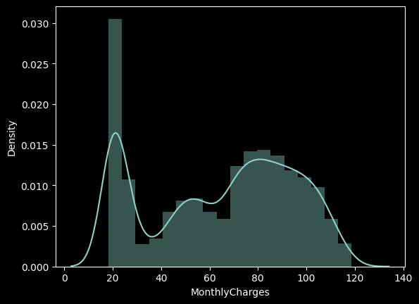
MonthlyCharges은 우수 고객 즉, 프리미엄 회원의 가입 요금을 의미하며 총 20 ~ 120 달러까지 요금을 내고 가입한 회원들이 존재하는 것으로 보인다. 구간화를 통해서 MonthlyCharges을 그룹핑하여 각 회원의 납부 요금 별로 이탈률을 계산해보자.
# ▶ 구간화
import numpy as np
df['MonthlyCharges_gp'] = np.where (df['MonthlyCharges'] <= 40, '40 이하',
                           np.where(df['MonthlyCharges'] <= 80, '40-80 이하', '80 초과'))

df[['MonthlyCharges','MonthlyCharges_gp']].head(5)

	MonthlyCharges	MonthlyCharges_gp
0			 29.85			   40 이하
1			 56.95	        40-80 이하
2			 53.85			40-80 이하
3			 42.30			40-80 이하
4			 70.70			40-80 이하
# ▶ 프리미엄 요금 회원들이 이탈률이 더 높다.
df_gp = df.groupby('MonthlyCharges_gp')['Churn'].agg(['count','sum'])
df_gp['ratio'] = round((df_gp['sum'] / df_gp['count']) * 100, 1)
df_gp['lift'] = round(df_gp['ratio'] / 27,1)
df_gp
count sum ratio lift
tenure_gp
40 이하 1838 214 11.6 0.4
40-80 이하 2539 749 29.5 1.1
80 초과 2666 906 34.0 1.3
구간화를 통해 확인해본 결과 프리미엄 요금을 내는 회원들의 ratio 즉 이탈률이 높은 것을 확인해볼 수 있으며 요금을 적개 내는 회원들의 이탈률이 낮은 것을 확인할 수 있어다.
이탈률이 27프로인것에 비해서 각 요금 그룹별로 몇배 더 이탈률이 높은 것인지 확인해본 결과 80 이상의 요금을 내는 고객의 이탈률이 1.3배나 높은 것을 확인할 수 있다.
그래서 프리미엄 고객의 이탈률이 많아지는 이유에 대해서 생각해볼 필요가 있다.
# ▶ 이용개월수 및 프리미엄 요금 회원 조합에 따른 이탈률 분석
df_gp = df.groupby(['tenure_gp','MonthlyCharges_gp'])['Churn'].agg(['count','sum'])
df_gp['ratio'] = round((df_gp['sum'] / df_gp['count']) * 100, 1)
df_gp

							  count	sum	ratio
tenure_gp	MonthlyCharges_gp
20 이하			40 이하		 873  187  21.4
				40-80 이하	 1300  597  45.9
				  80 초과	      705  467	66.2
20-60 이하		 40 이하	     674   26	3.9
				40-80 이하	  922  140	15.2
				  80 초과		 1162  359	30.9
60 초과			40 이하		 291	1   0.3
				40-80 이하	  317	12	 3.8
				 80 초과	      799	80	10.0
이용개월수 및 프리미엄 요금 회원 조합에 따른 이탈률 분포에 대해서도 함께 확인해보았다.
가입 개월 수를 기준으로 프리미엄 요금 회원 조합에 따라서도 프리미엄 회원 가입자의 이탈률이 높은 것을 확인할 수 있다.
이탈 고객 특성 분석
고객의 이탈률의 분포에 대한 정보는 대략적으로 확인해보았으며 그렇다면 이탈을 하는 고객의 개별적 특성을 분석해 이탈하는 고객을 분류해보고자 한다. 아래의 세 가지를 분석할 것이다.
**인구통계학적 특성 - 이탈률 분석
부가서비스 사용 - 이탈률 분석
계약 형태, 요금 - 이탈률 분석**
(1) 인구통계학적 특성 - 이탈률 분석
먼저 전체 데이터에서 고객의 개별적 특성을 나타낼만한 데이터들인 별/실버고객/결혼여부/부양가족여부를 데이터 프레임화 한 후 막대 그래프로 분포를 확인해 보았다.
# ▶ 인구통계학적 특성 성별/실버고객/결혼여부/부양가족여부
df[['gender', 'SeniorCitizen', 'Partner', 'Dependents']].head(10)

	gender	SeniorCitizen	Partner	Dependents
0	Female				0		Yes			No
1	  Male				0		No			No
2	  Male				0		No			No
3	  Male				0		No			No
4	Female				0		No			No
5	Female				0		No			No
6	  Male				0		No		   Yes
7	Female				0		No			No
8	Female				0		Yes			No
9	  Male				0		No		   Yes
# ▶ gender(성별)
sns.catplot(x="gender", hue="Churn", kind="count",palette="pastel", edgecolor=".6",data=df);
plt.gcf().set_size_inches(10, 3)
df_gp = df.groupby('gender')['Churn'].agg(['count','sum'])
df_gp['ratio'] = round((df_gp['sum'] / df_gp['count']) * 100, 1)
df_gp['lift'] = round(df_gp['ratio'] / ((df['Churn'].sum() / len(df))*100) ,1)
print(df_gp)
count sum ratio lift
gender
Female 3488 939 26.9 1.0
Male 3555 930 26.2 1.0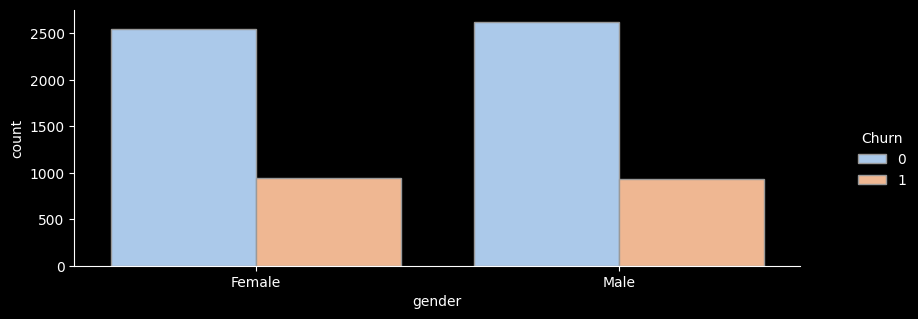
- 성별 이탈률을 확인해보니 성별 이탈률의 차이는 거의 동일하여 큰 의미가 없는 것으로 보인다.
# ▶ SeniorCitizen(노인가구여부)
sns.catplot(x="SeniorCitizen", hue="Churn", kind="count",palette="pastel", edgecolor=".6",data=df);
plt.gcf().set_size_inches(10, 3)


df_gp = df.groupby('SeniorCitizen')['Churn'].agg(['count','sum'])
df_gp['ratio'] = round((df_gp['sum'] / df_gp['count']) * 100, 1)
df_gp['lift'] = round(df_gp['ratio'] / ((df['Churn'].sum() / len(df))*100) ,1)
print(df_gp)

			   count   sum  ratio  lift
SeniorCitizen
0               5901  1393   23.6   0.9
1               1142   476   41.7   1.6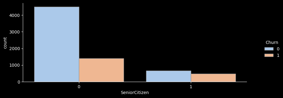
- 노인가구별 이탈률을 확인해보니 노인가구에 해당하는 가입자가 훨씬 더 높은 이탈률을 보이고 있는 것을 확인해볼 수있다.
# ▶ Partner(결혼여부)
sns.catplot(x="Partner", hue="Churn", kind="count",palette="pastel", edgecolor=".6",data=df);
plt.gcf().set_size_inches(10, 3)


df_gp = df.groupby('Partner')['Churn'].agg(['count','sum'])
df_gp['ratio'] = round((df_gp['sum'] / df_gp['count']) * 100, 1)
df_gp['lift'] = round(df_gp['ratio'] / ((df['Churn'].sum() / len(df))*100) ,1)
print(df_gp)

 		 count   sum  ratio  lift
Partner
No        3641  1200   33.0   1.2
Yes       3402   669   19.7   0.7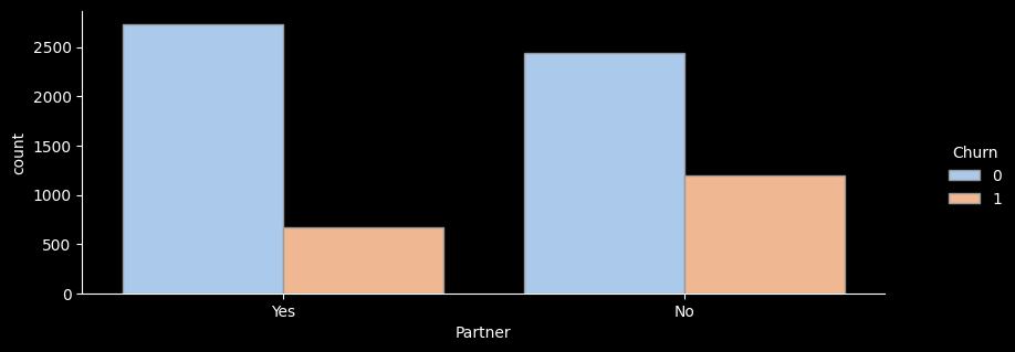
- 결혼여부별 이탈률을 확인해보니 미혼자에 해당하는 가입자가 훨씬 더 낮은 이탈률을 보이고 있는 것을 확인해볼 수있다.
# ▶ Dependents(부양가족 여부)
sns.catplot(x="Dependents", hue="Churn", kind="count",palette="pastel", edgecolor=".6",data=df);
plt.gcf().set_size_inches(10, 3)


df_gp = df.groupby('Dependents')['Churn'].agg(['count','sum'])
df_gp['ratio'] = round((df_gp['sum'] / df_gp['count']) * 100, 1)
df_gp['lift'] = round(df_gp['ratio'] / ((df['Churn'].sum() / len(df))*100) ,1)
print(df_gp)

 		 	count   sum  ratio  lift
Dependents
No           4933  1543   31.3   1.2
Yes          2110   326   15.5   0.6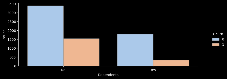
- 부양가족이 있는지 별로 이탈률을 확인해보니 부양가족이 없음에 해당하는 가입자가 훨씬 더 높은 이탈률을 보이고 있는 것을 확인해볼 수있다.
(2) 부가서비스 사용 - 이탈률 분석
먼저 전체 데이터에서 가입 시 부가서비스를 이용하는지 확인할 수 있는 데이터들인 온락인백업서비스/기기보험서비스/기술지원서비스/스트리밍TV/스트리밍영화 서비스데이터 프레임화 한 후 막대 그래프로 분포를 확인해 보았다.
# ▶ 부가서비스 col, 온락인백업서비스/기기보험서비스/기술지원서비스/스트리밍TV/스트리밍영화 서비스
df[['OnlineBackup', 'DeviceProtection', 'TechSupport', 'StreamingTV', 'StreamingMovies']]

	OnlineBackup	DeviceProtection	TechSupport	StreamingTV	StreamingMovies
0			 Yes				  No			 No			 No				 No
1			  No				 Yes			 No			 No				 No
2			 Yes				  No			 No			 No				 No
3			  No				 Yes			Yes			 No				 No
4			  No				  No			 No			 No				 No
# ▶ for문 활용 한 번에 출력
col_list = ['OnlineBackup', 'DeviceProtection', 'TechSupport', 'StreamingTV', 'StreamingMovies']
for i in col_list :
val = i
sns.catplot(x=val, hue="Churn", kind="count",palette="pastel", edgecolor=".6",data=df);
plt.gcf().set_size_inches(10, 3)
df_gp = df.groupby(val)['Churn'].agg(['count','sum'])
df_gp['ratio'] = round((df_gp['sum'] / df_gp['count']) * 100, 1)
df_gp['lift'] = round(df_gp['ratio'] / ((df['Churn'].sum() / len(df))*100) ,1)
print(df_gp)
print("---------------------------------------")
count sum ratio lift
OnlineBackup
No 3088 1233 39.9 1.5
No internet service 1526 113 7.4 0.3
Yes 2429 523 21.5 0.8
---------------------------------------
count sum ratio lift
DeviceProtection
No 3095 1211 39.1 1.5
No internet service 1526 113 7.4 0.3
Yes 2422 545 22.5 0.8
---------------------------------------
count sum ratio lift
TechSupport
No 3473 1446 41.6 1.6
No internet service 1526 113 7.4 0.3
Yes 2044 310 15.2 0.6
---------------------------------------
count sum ratio lift
StreamingTV
No 2810 942 33.5 1.3
No internet service 1526 113 7.4 0.3
Yes 2707 814 30.1 1.1
---------------------------------------
count sum ratio lift
StreamingMovies
No 2785 938 33.7 1.3
No internet service 1526 113 7.4 0.3
Yes 2732 818 29.9 1.1
---------------------------------------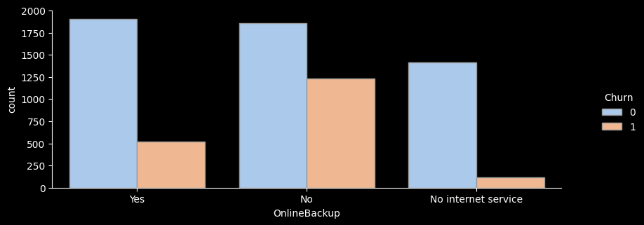
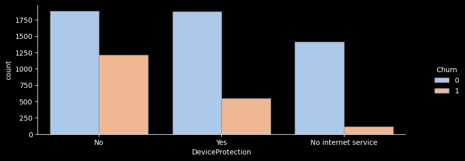
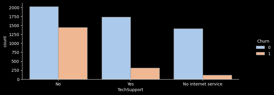
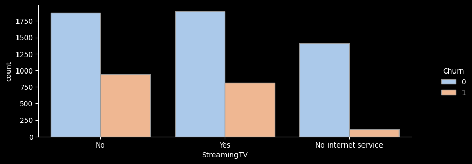
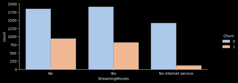
- for문을 활용해 온락인백업서비스/기기보험서비스/기술지원서비스/스트리밍TV/스트리밍영화 서비스 의 이탈률을 한눈에 그래프로 확인해보았다.
- 전체적으로 서비스를 이용하지 않는 고객의 이탈률이 가장 높은 것으로 나타난다.
- 하지만 스트리밍 서비스, 스트리밍 영화 서비스를 이용하는 고객이나 이용하지 않는 고객의 이탈률은 크게 차이가 나지 않는 것으로 보인다.
그래서 전체적으로 부가서비스를 아예 이용하지 않는 고객의 이탈률이 낮은 것을 확인하기 위해 이탈률을 확인해보니
# ▶ 부가서비스를 모두 이용하지 않는 고객에 이탈률 분석
df_no = df[(df['OnlineBackup'] =='No') & (df['DeviceProtection'] =='No') & (df['TechSupport'] =='No') & (df['StreamingTV'] =='No') & (df['StreamingMovies'] =='No')]
df_no[col_list]

	OnlineBackup	DeviceProtection	TechSupport	StreamingTV	StreamingMovies
4			  No				  No			 No			 No				 No
7			  No				  No			 No			 No				 No
10			  No				  No			 No			 No				 No
36			  No				  No			 No			 No				 No
...	...	...	...	...	...
7026		  No				  No			 No			 No				 No
7032		  No				  No			 No			 No				 No
7033		  No				  No			 No			 No				 No
7040		  No				  No			 No			 No				 No
7041		  No				  No			 No			 No				 No
# ▶ 부가서비스 형태가 모두 No인고객은 47.6% 이탈률, Lift 약 1.8
df_no['Churn'].sum() / len(df_no)- 그래서 부가서비스를 모두 이용하지 않는 고객에 이탈률을 분석해본 결과 부가서비스를 모두 이용하지 않는 고객의 이탈률이 모두 47.6%로 절반을 보이며 부가서비스를 이용하지 않는 고객들의 이탈률이 상당히 높은 것을 확인할 수 있었다.
(3) 계약 형태, 요금 - 이탈률 분석
다음으로는 전체 데이터에서 계약형태를 확인할 수 있는 데이터들인 계약기간/종이없는청구/결제수단 등의 데이터를 데이터 프레임화 한 후 분포를 확인해보았다.
# ▶ 계약형태 col, 계약기간/종이없는청구/결제수단
df[['Contract', 'PaperlessBilling', 'PaymentMethod']]

		  	Contract	PaperlessBilling	   			PaymentMethod
0	  Month-to-month				 Yes			 Electronic check
1		    One year				  No				 Mailed check
2	  Month-to-month				 Yes				 Mailed check
3		    One year				  No	Bank transfer (automatic)
4	  Month-to-month				 Yes			 Electronic check
...				 ...				 ...						  ...
7038	    One year				 Yes				 Mailed check
7039	    One year				 Yes	  Credit card (automatic)
7040  Month-to-month				 Yes	  		 Electronic check
7041  Month-to-month				 Yes				 Mailed check
7042	    Two year				 Yes	Bank transfer (automatic)
# ▶ for문 활용 한 번에 출력
col_list = ['Contract', 'PaperlessBilling', 'PaymentMethod']
for i in col_list :
val = i
df_gp = df.groupby(val)['Churn'].agg(['count','sum'])
df_gp['ratio'] = round((df_gp['sum'] / df_gp['count']) * 100, 1)
df_gp['lift'] = round(df_gp['ratio'] / ((df['Churn'].sum() / len(df))*100) ,1)
print(df_gp)
print("---------------------------------------------------")
count sum ratio lift
Contract
Month-to-month 3875 1655 42.7 1.6
One year 1473 166 11.3 0.4
Two year 1695 48 2.8 0.1
---------------------------------------------------
count sum ratio lift
PaperlessBilling
No 2872 469 16.3 0.6
Yes 4171 1400 33.6 1.3
---------------------------------------------------
count sum ratio lift
PaymentMethod
Bank transfer (automatic) 1544 258 16.7 0.6
Credit card (automatic) 1522 232 15.2 0.6
Electronic check 2365 1071 45.3 1.7
Mailed check 1612 308 19.1 0.7
---------------------------------------------------- 확인 결과 월 단위 가입자의 이탈률이 당연히 높은 것을 확인 할 수 있다.
- 종이 청구서를 이용하지 않는 고객의 이탈률이 더 높은 것을 확인할 수 있다.
Electonice check를 이용해 결제하는 고객의 이탈률이 가장 많이 높은 것을 확인할 수 있다.
결론
-
넷플릭스는 최근 몇 년 동안 급성장세를 보였으며 2016년을 시작으로 2020년까지 다수의 컨텐츠를 제작하고 있는 것을 확인했다.
-
12월에 가장 많은 컨텐츠가 추가되었으며, 10월 1월에도 비슷한 수준이지만 상대적으로 다른 월에 비해 많은 컨텐츠가 추가된 것을 확인할 수 있다.
-
그래서 10월~내년도 1월까지 특히 연말에 컨텐츠 추가가 집중되는 경향이 있는 것으로 보인다. 이는 연말 시즌에 맞춘 콘텐츠 업데이트 전략을 반영할 수 있을 것으로 보인다.
-
넷플릭스에서 제작된 컨텐츠들은 티비쇼보다는 영화 제작에 더 집중을 하고 있으며 컨텐츠는 대부분을 성인을 타깃으로 하는 컨텐츠를 제작한 것으로 보인다.
-
영화 컨텐츠의 제작 길이는 80분에서 120분 사이의 길이를 가지고 있어 극장 영화보다 짧은 시간의 길이를 가지고 있다.
-
아무래도 미국 회사다 보니 미국이 압도적으로 컨텐츠 제작이 많으며 그 다음은 영화산업이 발달 돼 있는 인도가 위치해 있으며 그 다음으로 영국, 일본이 뒤를 이었다. 이는 넷플릭스의 컨텐츠가 주로 이 세 국가에서 제작됐음을 확인할 수 있다.
- 장르별 컨텐츠의 분포를 확인해보니 가장 인기 있는 장르는
'International Movies'국제 영화와'Dramas'드라마로 나타났디. 이는 넷플릭스가 국제적인 시청자를 대상으로 다양한 영화를 제공하고 있음을 시사한다.