Experiments

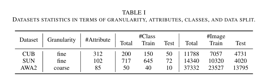
DATASETS STATISTICS IN TERMS OF GRANULARITY, ATTRIBUTES, CLASSES, AND DATA SPLIT
GRANULARITY 세분성
세분성, 속성, 클래스 및 데이터 분할 측면에서 데이터셋 통계

A. Dataset and evaluation metrics

We evaluate our method on three most widely used datasets CUB [28], SUN [29] and AwA2 [30], and follow the proposed train and test split in [30].
우리는 가장 널리 사용되는 세 가지 데이터 세트 CUB [28], SUN [29] 및 AwA2 [30]에 대해 우리의 방법을 평가하고 [30]에서 제안된 트레인 및 테스트 분할을 따릅니다.

The statistics of the datasets is summarized in Table I: Caltech-UCSD Birds-200-2011 (CUB) [28] is the most fine-grained dataset with 312 attributes.
데이터 세트의 통계는 표 I에 요약되어 있습니다. Caltech-UCSD Birds-200-2011(CUB)[28]은 312개의 속성을 가진 가장 세분화된 데이터 세트입니다.

It contains 11788 images with 150 seen classes and 50 unseen classes.
150개의 본 클래스와 50개의 보이지 않는 클래스가 있는 11788개의 이미지가 포함되어 있습니다.

SUN [29] is a large scene dataset which has 14340 images with 645 seen classes and 72 unseen classes.
scene 장면
SUN [29]은 645개의 보이는 클래스와 72개의 보이지 않는 클래스가 있는 14340개의 이미지가 있는 대규모 장면 데이터 세트입니다.

There are 102 attributes in total.
총 102개의 속성이 있습니다.

Compared with the former two, AwA2 [30] is a relatively coarse dataset with only 85 attributes but it has the 37332 images which is the most of three datasets.
coarse 거친, 조잡한
AwA2[30]는 앞의 두 가지에 비해 속성이 85개에 불과한 비교적 조잡한 데이터셋이지만 3개 데이터셋 중 가장 많은 37332개의 이미지를 가지고 있다.

It contains 40 seen classes and 10 unseen classes.
그것은 40개의 본 클래스와 10개의 보이지 않는 클래스를 포함합니다.

---

We report results in both ZSL and GZSL settings (Sec. III-A).
ZSL 및 GZSL 설정(섹션 III-A) 모두에서 결과를 보고합니다.

In the ZSL setting, we only evaluate the performance on unseen classes and use the top-1 accuracy (T1) as the evaluation metric.
ZSL 설정에서는 보이지 않는 클래스에 대한 성능만 평가하고 평가 메트릭으로 최상위 정확도(T1)를 사용합니다.

In the GZSL setting, we evaluate the performance on both seen and unseen classes and follow [30] to use generalized seen accuracy ($Acc_S$), generalized unseen accuracy ($Acc_U$) and their generalized Harmolic Mean($Acc_H$) as evaluate metrics.
GZSL 설정에서 우리는 보이는 클래스와 보이지 않는 클래스 모두에 대한 성능을 평가하고 [30]에 따라 일반화된 본 정확도($Acc_S$), 일반화된 보이지 않는 정확도($Acc_U$) 및 일반화된 조화 평균($Acc_H$)을 평가 메트릭으로 사용합니다.

The former two are top-1 accuracy for seen and unseen classes respectively while the last one is obtained by,
앞의 두 가지는 보이는 클래스와 보이지 않는 클래스에 대해 각각 최고 1 정확도이고 마지막 클래스는 다음과 같이 얻습니다.

$Acc_H$ measures the inherent bias towards seen classes [52], which is a more important metric in GZSL.
inherent 고유의

B. Implementation details

As a default backbone, we choose the CNN-based architecture, ResNet101 [3], which is pre-trained on ImageNet1k (1.28 million images, 1000 classes).
기본 백본으로 ImageNet1k(128만 이미지, 1000개 클래스)에서 사전 훈련된 CNN 기반 아키텍처인 ResNet101[3]을 선택합니다.

The input image resolution is 448 × 448 and global feature cf is of 2048 dimensions.
입력 이미지 해상도는 448 × 448이고 전역 기능 cf는 2048 차원입니다.

For transformer-based architecture, the large variant of the vision transformer (ViT) [49] is used, which is pre-trained on ImageNet21k (14 million images, 21,843 classes).
트랜스포머 기반 아키텍처의 경우 ImageNet21k(1400만 이미지, 21843 클래스)에서 사전 훈련된 ViT(Vision Transformer)[49]의 큰 변형이 사용됩니다.

The input image resolution is 224 × 224 and global feature cf is of 1024 dimensions; the patch size is 16 × 16, such that there are 196 patch tokens in total.
입력 이미지 해상도는 224 × 224이고 전역 기능 cf는 1024 차원입니다. 패치 크기는 16 × 16이므로 총 196개의 패치 토큰이 있습니다.

The hidden size of prototype generation module is set to 1024. τ in (5) is set to 0.4 for CUB, 0.6 for SUN and AwA2.
프로토타입 생성 모듈의 숨겨진 크기는 1024로 설정됩니다. (5)의 τ는 CUB의 경우 0.4, SUN 및 AwA2의 경우 0.6으로 설정됩니다.

β in (4) is set to 0.5 and α in (1) is 25 for all datasets. λ attp , λ attf , λ sem in (7) is set as 0.1, 1 and 1, respectively.
(4)의 β는 0.5로 설정되고 (1)의 α는 모든 데이터 세트에 대해 25입니다. (7)에서 λ attp , λ attf , λ sem 은 각각 0.1, 1, 1로 설정된다.

We choose the SGD optimizer and set the momentum as 0.9, initial learning rate 0.001, and weight decay 0.0001.
SGD 옵티마이저를 선택하고 운동량을 0.9, 초기 학습률 0.001, 가중치 감소 0.0001로 설정합니다.

The learning rate is decayed every 10 epochs, with the decay factor of 0.5.
학습률은 10 Epoch마다 감쇠되며 감쇠 계수는 0.5입니다.

All models are trained with synchronized SGD over 4 GPUs for 20 epochs with a mini-batch of 32.
synchronized 동기화된
모든 모델은 32개의 미니 배치로 20개의 에포크 동안 4개의 GPU를 통해 동기화된 SGD로 훈련됩니다.

The mini-batch is organized as a 16-way 2-shot episode following [13] meaning that we sample 2 images per class for 16 classes within this mini-batch.
미니 배치는 [13]에 이어 16방향 2샷 에피소드로 구성됩니다. 즉, 이 미니 배치 내에서 16개 클래스에 대해 클래스당 2개의 이미지를 샘플링합니다.