Boosting Zero-shot Learning via Contrastive Optimization of Attribute Representations 제5-3부 method

이준석·2022년 7월 28일

Boosting Zero-shot Learning via constrastive Optimization of Attribute Representations

목록 보기

12/12

E. Parameter variation

1) Temperature τ in Eq. (5):

In Fig. 3, we evaluate the effect of temperature τ in Eq. (5).
그림 3에서 우리는 Eq.에서 온도 τ의 영향을 평가합니다. (5).

We vary it from 0.05 to 1 on the three datasets and report the T1 and $Acc_H$ for ZSL and GZSL, respectively.
vary 다르다 달라지다, 변경하다
3개의 데이터 세트에서 0.05에서 1로 변경하고 ZSL 및 GZSL에 대해 각각 T1 및 $Acc_H$ 를 보고합니다.

It can be seen that the best performance occurs with τ equivalent to 0.4 and 0.6 for CUB and AwA2, respectively.
CUB 및 AwA2에 대해 각각 0.4 및 0.6에 해당하는 τ에서 최상의 성능이 발생함을 알 수 있습니다.

The performance on SUN is rather stable by varying τ.
SUN 의 성능은 τ 를 변경함으로써 다소 안정적입니다.

A low temperature will penalize more on hard negatives but a too low temperature will make no tolerance for outliers which can not be a good thing.
tolerance 허용오차 outliers 특이값, 이상치

In practice, we set τ as 0.4 for CUB and 0.6 for SUN and AwA2.
실제로 τ를 CUB의 경우 0.4로 설정하고 SUN 및 AwA2의 경우 0.6으로 설정합니다.

2) Scaling factor α in Eq. (1):

We show the impact of scaling factor α in Eq(1) by varying it from 20 to 30 in Fig4.
그림 4에서 20에서 30으로 변화시켜 식(1)에서 스케일링 인자 α의 영향을 보여줍니다.

CoAR-ZSL achieves the best performance on CUB at α = 25 for both T1 and $Acc_H$ .
CoAR-ZSL은 T1 및 $Acc_H$ 모두에 대해 α = 25에서 CUB에서 최고의 성능을 달성합니다.

For SUN and AwA2, the performance variation with different α is rather small on both T1 and $Acc_H$ .
SUN 및 AwA2의 경우 T1 및 AccH 모두에서 α가 다른 성능 변동이 다소 작습니다.

In practice, we set α as 25 for all datasets for simplicity.
실제로 단순화를 위해 모든 데이터 세트에 대해 α를 25로 설정했습니다.

3) Ratio β in Eq. (4):

We also evaluate the effect of ratio β in Eq(4).
우리는 또한 Eq(4)에서 비율 β의 효과를 평가합니다.

We plot the result in Fig5.

CoAR-ZSL achieves the best performance on CUB at β = 0.5 for both T1 and $Acc_H$ .
CoAR-ZSL은 T1 및 $Acc_H$ 모두에 대해 β = 0.5에서 CUB에서 최고의 성능을 달성합니다.

For SUN and AwA2, the performance variation with different β is rather small on both T1 and $Acc_H$ .
SUN 및 AwA2의 경우 β가 다른 성능 변동은 T1과 $Acc_H$ 모두에서 다소 작습니다.

In practice, we set β as 0.5 for all datasets for simplicity.
실제로 단순화를 위해 모든 데이터 세트에 대해 β를 0.5로 설정했습니다.

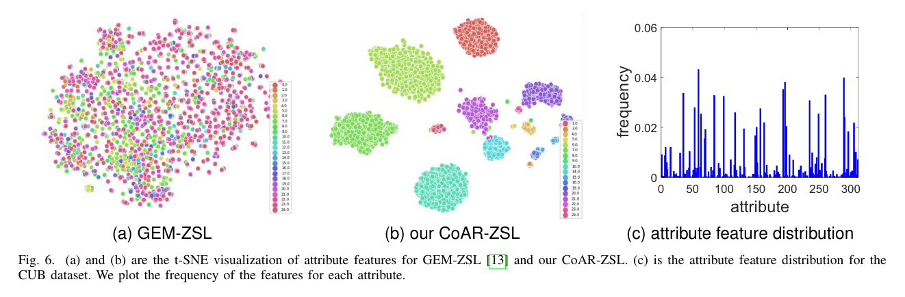
Fig 6. (a) and (b) are the t-SNE visualization of attribute features for GEM-ZSL [13] and our CoAR-ZSL.
(a) 및 (b)는 GEM-ZSL [13] 및 CoAR-ZSL에 대한 속성 기능의 t-SNE 시각화입니다.
(c) is the attribute feature distribution for the CUB dataset.
(c)는 CUB 데이터 세트에 대한 속성 특성 분포입니다.
We plot the frequency of the features for each attribute.
각 속성에 대한 기능의 빈도를 표시합니다.

Fig 7. Visualization of intermediate feature maps in Eq(3).
Eq(3)에서 중간 기능 맵의 시각화.

F. Qualitative results

1) Attribute localization:

To visualize the attention-based attribute localization (Sec. III-D), we resize and normalize the attribute-related attention maps in AM into the range [0,1] and draw them onto the original image in Fig8.
주의 기반 속성 지역화(Sec. III-D)를 시각화하기 위해 AM의 속성 관련 주의 맵의 크기를 조정하고 [0,1] 범위로 정규화하고 그림 8의 원본 이미지에 그립니다.

We show the examples using both the CNN-based and transformer-based architectures. In both figures, CoAR-ZSL can accurately locate attribute-related regions in images.
CNN 기반 및 변압기 기반 아키텍처를 모두 사용하여 예제를 보여줍니다. 두 그림에서 CoAR-ZSL은 이미지에서 속성 관련 영역을 정확하게 찾을 수 있습니다.

2) The intermediate feature maps in Eq.(3):

2) Eq.(3)의 중간 기능 맵:

We illustrate the intermediate feature maps after fusion of intermediate layers, after softmax, and after fusion with the image feature tensor F.
fusion 중간, intermediate 중간의
중간 레이어 융합 후, 소프트맥스 이후, 이미지 특징 텐서 F와의 융합 후 중간 특징 맵을 설명한다.

Referring to Eq(3), they correspond to the feature map $am_j$ , $Softmax(am_j)$ , and $R(Softmax(am_j)) \odot F$ , respectively.
Eq(3)을 참조하면 각각 $am_j$ , $Softmax(am_j)$ 및 $R(Softmax(am_j)) \odot F$ 기능 맵에 해당합니다.

We draw the attribute “has bill shape dagger” in Fig. 7: one can clearly observe how this attribute is localized in F via the corresponding normalized soft mask $(Softmax(amj))$ .
우리는 그림 7에 "hall shape dagger"라는 속성을 그렸습니다. 이 속성이 해당 정규화된 소프트 마스크 $(Softmax(amj))$ 를 통해 F에 어떻게 지역화되어 있는지 명확하게 관찰할 수 있습니다.

It aligns with the attribute on the bird’s beak.
align 일치하다
새 부리의 속성과 일치합니다.

3) t-SNE visualization of attribute features:

To validate the representativeness of the proposed attribute-level features, we draw the t-SNE of 4096 attribute-level features extracted over multiple images using methods of both our CoAR-ZSL (Fig6b) and GEM-ZSL (13) (Fig6a).
validate 검증하다 multiple 여러장
제안된 속성 수준 특징의 대표성을 검증하기 위해 CoAR-ZSL(그림 6b)과 GEM-ZSL(13)(그림 6a)의 방법을 사용하여 여러 이미지에서 추출된 4096 속성 수준 특징의 t-SNE를 그립니다.

For better visualization, we only plot the first 25 attributes in different colors.
더 나은 시각화를 위해 처음 25개의 속성만 다른 색상으로 표시합니다.

We can see that the attribute-level features in our model are clearly clustered according to the attribute they belong to while the ones in GEM-ZSL are rather mixed.
우리 모델의 속성 수준 기능은 속한 속성에 따라 명확하게 클러스터링된 반면 GEM-ZSL의 기능은 다소 혼합되어 있음을 알 수 있습니다.

Since we only keep attribute-level features with high peak values in their corresponding attribute-related attention maps ( $AM$ ), it can be seen the kept features tend to form a number of big clusters for a number of attributes.
해당 속성 관련 주의 맵( $AM$ )에서 피크 값이 높은 속성 수준 기능만 유지하기 때문에 유지된 기능은 여러 속성에 대해 많은 큰 클러스터를 형성하는 경향이 있음을 알 수 있습니다.

This is indeed consistent to the attribute feature distribution shown in Fig6c: only a number of attributes have high frequencies.
이것은 실제로 그림 6c에 표시된 속성 특성 분포와 일치합니다. 일부 속성에만 높은 빈도가 있습니다.

The similar observation is made in [31] that many fine-grained classes contain discriminative information in a few regions.
유사한 관찰은 [31]에서 많은 세분화된 계층이 일부 지역의 차별적 정보를 포함하고 있다는 것이다.

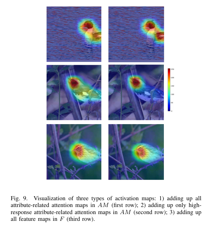
Fig. 9. Visualization of three types of activation maps: 1) adding up all attribute-related attention maps in AM (first row); 2) adding up only highresponse attribute-related attention maps in AM (second row); 3) adding up all feature maps in F (third row).
그림 9. 세 가지 유형의 활성화 맵 시각화: 1) AM(첫 번째 행)에서 모든 속성 관련 주의 맵을 합산합니다. 2) AM(두 번째 행)에서 고응답 속성 관련 주의 맵만 추가합니다. 3) F(세 번째 행)의 모든 기능 맵을 합산합니다.

4) Qualitative evidence for selecting high-response attention maps for constrastive optimization:

Qulitative 점성적
4) 콘트라스트 최적화를 위한 높은 응답 주의 맵을 선택하기 위한 정성적 근거:

We plot three types of activation maps in Fig9 in three rows: 1) adding up all attribute-related attention maps in AM ; 2) adding up only high-response attribute-related attention maps in AM ; 3) adding up all feature maps in F.
우리는 그림 9에서 세 가지 유형의 활성화 맵을 세 행으로 표시합니다. 1) AM의 모든 속성 관련 주의 맵을 합산합니다. 2) AM에서 고응답 속성 관련 주의 맵만 추가합니다. 3) F의 모든 기능 맵을 합산합니다.

We know that each attention map $am_j$ in AM signifies the feature response to one attribute j.
AM의 각 어텐션 맵 $am_j$ 는 하나의 속성 j에 대한 기능 응답을 의미한다는 것을 알고 있습니다.

Adding them together can be a reflection of these attributes on certain object class.
이들을 함께 추가하면 특정 객체 클래스에서 이러한 속성을 반영할 수 있습니다.

On the other hand, since the class-level feature cf is actually obtained from F , adding all feature maps in F is indeed a reflection of the object class in the image.
반면에 클래스 레벨 피쳐 cf는 실제로 F로부터 얻어지기 때문에 F의 모든 피쳐 맵을 추가하는 것은 실제로 이미지의 객체 클래스를 반영하는 것이다.

Having a look at Fig. 9, activation maps in the second row are clearly cleaner and more object-focused than those in the first row, and are visually closer to those in the third row.
그림 9를 보면 두 번째 행의 활성화 맵이 첫 번째 행보다 명확하고 객체 중심적이며 시각적으로 세 번째 행에 더 가깝습니다.

This suggests that there exist noises in those low-response attention maps in AM which could be brought into the activation map if adding them up.
이것은 AM의 저응답 주의 맵에 노이즈가 있음을 시사하며, 이를 합산하면 활성화 맵으로 가져올 수 있습니다.

While those high-response attention maps in AM represent the real attributes contained in the object class, adding these maps can end up with a proper reflection of attributes on this object class.
AM의 고응답 주의 맵은 객체 클래스에 포함된 실제 속성을 나타내지만 이러한 맵을 추가하면 이 객체 클래스의 속성이 적절히 반영될 수 있습니다.

이준석

인공지능 전문가가 될레요

이전 포스트