1. 이론

기계가 미지의 함수(black-box)를 배우는 방법은?

• 가장 대중적인 방법 중 하나는 미분(derivative)를 구하는 것

편미분

• $f(x)$와 같은 한개의 변수가 아닌 다변수 함수의 미분을 말한다.
  (즉, 현실에는 변수가 한개인 경우가 거의 없기 때문)

• $f(x,y,z,...)$ 등으로 표기할 수 있음.

• 일반적으로 굉장히 많은 변수들이 있을 때는 $f(x_1,x_2,...,x_n)$ 의 n개 다변수함수로 표현 할 수 있음.

• Partial derivative라고 부름.

• $z=f(x,y)$ 표현된다면 각각의 편미분은 $\frac{\partial z}{\partial x}$ ($x$에 대해 미분), $\frac{\partial z}{\partial y}$ ($y$에 대해 미분)로 표기함.

• 다변수함수($f(x_1, x_2, ... , x_n)$에 대해 각각의 편미분을 $\frac{\partial f}{\partial x_i}$로 표기함.

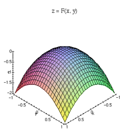
편미분의 기하학적 의미

• $z = f(x,y)$는 $x,y,z$축의 3차원 위의 평면/곡면을 나타냄.
• $(x,y) = (0,0)$에서 아래 곡면에 접하는 평면을 구하고자 함.
• $(0,0)$에서 각 변수 x와 y에 대한 편미분을 통해 접선을 구하고, 이를 활용해 평면을 구함.
• 접선의 확장임.
  

2. 코드 실습

2-1. Gradient Descent 다항함수

다항 함수의 gradient descent를 구합니다.

x=3에서 부터 lr=0.01을 통해서 이동하여 최저점을 구합니다. 최대 10,000번을 이동합니다.
x의 입력이 들어왔을 때 $(x+5)^2$ 의 출력을 내는 함수를 선언합니다.

def main():
    
    gradient()
    
def gradient():
    cur_x = 3                       # 현재 x
    lr = 0.01                       # Learning rate
    threshold = 0.000001            # 알고리즘의 while문을 조절하는 값.
    previous_step_size = 1 
    max_iters = 10000               # 최대 iteration 횟수
    iters = 0 #iteration counter
    f = lambda x : (x+5)**2
    df = lambda x : 2*(x+5)        # 구하고자하는 함수의 미분함수
    
    while previous_step_size > threshold and iters < max_iters:
        prev_x = cur_x                               # 현재 x를 prev로 저장합니다.
        cur_x = cur_x - lr * df(prev_x)              # Grad descent를 합니다.
        previous_step_size = abs(cur_x - prev_x)      #x의 변화량을 구합니다.
        iters = iters+1 #iteration count
        print("Iteration",iters,"\nx 값은 ",cur_x, "\ny 값은 ", f(cur_x))           #Print iterations

if __name__ == "__main__":
    main()

2-2. Gradient Descent 지수함수

지수 함수의 gradient descent를 구합니다.

x=3에서 부터 lr=0.01을 통해서 이동하여 최저점을 구합니다. 최대 10,000번을 이동합니다.
x의 입력이 들어왔을 때 $e^x$ 의 출력을 내는 함수를 선언합니다.

x,y를 저장해 plt.plot을 활용한 그림을 출력하세요.

def main():
    
    gradient()
    
def gradient():
    cur_x = 3                              # 현재 x
    lr = 0.01                              # Learning rate
    threshold = 0.000001                   # 알고리즘의 while문을 조절하는 값.
    previous_step_size = 1 
    max_iters = 10000                      # 최대 iteration 횟수
    iters = 0 #iteration counter
    f = lambda x: np.exp(x+1)               # 우리가 구하고자하는 함수의 미분함수
    df = lambda  x: np.exp(x+1)
    
    history_x = []
    history_y = []
    while previous_step_size > threshold and iters < max_iters:
        prev_x = cur_x                          # 현재 x를 prev로 저장합니다.
        cur_x = cur_x - lr * df(prev_x)         #Grad descent
        previous_step_size = abs(cur_x - prev_x) #x의 변화량을 구합니다.
        iters = iters+1 #iteration count
        print("Iteration",iters,"\nx 값은 ",cur_x, "\ny 값은 ", f(cur_x)) #Print iterations
        history_x.append(cur_x)
        history_y.append(f(cur_x))

    plt.plot(history_x, history_y, marker='o')
    plt.show()

if __name__ == "__main__":
    main()

2-3. Gradient Descent 로그

로그 함수의 gradient descent를 구합니다.

x=2에서 부터 lr=0.001을 통해서 이동하여 최저점을 구합니다. 최대 5,000번을 이동합니다.

def main():
    
    gradient()
    
def gradient():
    cur_x = 2                           # 현재 x
    lr = 0.001                          # Learning rate
    threshold = 0.000001                # 알고리즘의 while문을 조절하는 값.
    previous_step_size = 1 
    max_iters = 5000                    # 최대 iteration 횟수
    iters = 0 #iteration counter
    f = lambda x : np.log(x)
    df = lambda x: 1/x                  # 우리가 구하고자하는 함수의 미분함수
    
    history_x = []
    history_y = []
    while previous_step_size > threshold and iters < max_iters:
        prev_x = cur_x                      # 현재 x를 prev로 저장합니다.
        cur_x = cur_x - lr * df(prev_x)     # Grad descent를 합니다.
        previous_step_size = abs(cur_x - prev_x)    #x의 변화량을 구합니다.
        iters = iters+1 #iteration count
        print("Iteration",iters,"\nx 값은 ",cur_x, "\ny 값은 ", f(cur_x)) #Print iterations
        history_x.append(cur_x)
        history_y.append(f(cur_x))

    plt.plot(history_x, history_y, marker='o')
    plt.savefig("history.png")
    elice_utils.send_image("history.png")



if __name__ == "__main__":
    main()

2-4. 시험

from elice_utils import EliceUtils
import matplotlib.pyplot as plt
import numpy as np
import pandas as pd

elice_utils = EliceUtils()

np.random.seed(100)


def main():
    data = pd.read_csv('./data.csv', header=None)
    X = np.array(data[[0,1]])
    y = np.array(data[2])
    plot_points(X,y)

    plt.savefig("plot.png")
    elice_utils.send_image("plot.png")
    
    epochs = 100
    learnrate = 0.01
    train(X, y, epochs, learnrate, True)



def plot_points(X, y):
    admitted = X[np.argwhere(y==1)]
    rejected = X[np.argwhere(y==0)]
    plt.scatter([s[0][0] for s in rejected], [s[0][1] for s in rejected], s = 25, color = 'blue', edgecolor = 'k')
    plt.scatter([s[0][0] for s in admitted], [s[0][1] for s in admitted], s = 25, color = 'red', edgecolor = 'k')

def display(m, b, color='g--'):
    plt.xlim(-0.05,1.05)
    plt.ylim(-0.05,1.05)
    x = np.arange(-10, 10, 0.1)
    plt.plot(x, m*x+b, color)

    # Activation (sigmoid) function
def sigmoid(x):
    return 1 / (1 + np.exp(-x))

def function(features, weights, bias):
    return sigmoid(np.dot(features, weights) + bias)

def objective(y, output):
    return - y*np.log(output) - (1 - y) * np.log(1-output)

def update_weights(x, y, weights, bias, learnrate):
    output = sigmoid(np.dot(features, weights) + bias) # function 함수를 통해 나오는 출력을 적어주세요.
    d_error = -(y - output)
    weights -= learnrate*d_error*x # d_error * x는 gradient 값입니다. gradient에는 learning rate을 곱해주어서 weight를 업데이트 합니다.
    bias -= d_error*learnrate # weight와 마찬가지로 learningrate을 곱해서 update 해주세요.
    return weights, bias


def train(features, targets, epochs, learnrate, graph_lines=False):
    
    errors = []
    n_records, n_features = features.shape
    last_loss = None
    weights = np.random.normal(scale=1 / n_features**.5, size=n_features)
    bias = 0
    for e in range(epochs):
        del_w = np.zeros(weights.shape)
        for x, y in zip(features, targets):
            output = function(x, weights, bias)
            error = objective(y, output)
            weights, bias = update_weights(x, y, weights, bias, learnrate)
        
        # Printing out the log-loss error on the training set
        out = function(features, weights, bias)
        loss = np.mean(objective(targets, out))
        errors.append(loss)
        if e % (epochs / 10) == 0:
            print("\n========== Epoch", e,"==========")
            if last_loss and last_loss < loss:
                print(f"Train loss: {loss:.15f}  WARNING - Loss Increasing")
            else:
                print(f"Train loss: {loss:.15f}")
            last_loss = loss
            predictions = out > 0.5
            accuracy = np.mean(predictions == targets)
            print("Accuracy: ", accuracy)
        if graph_lines and e % (epochs / 10) == 0:
            display(-weights[0]/weights[1], -bias/weights[1])
            


    # Plotting the solution boundary
    plt.title("Solution boundary")
    display(-weights[0]/weights[1], -bias/weights[1], 'black')

    # Plotting the data
    plot_points(features, targets)
    plt.savefig("plot1.png")
    elice_utils.send_image("plot1.png")

    # Plotting the error
    plt.cla()
    plt.title("Error Plot")
    plt.xlabel('Number of epochs')
    plt.ylabel('Error')
    plt.plot(errors)

    plt.savefig("plot2.png")
    elice_utils.send_image("plot2.png")


if __name__ == "__main__":
    main()