1. Group

군(group)이란 어떤 집합과 연산자로 이루어져 있으며, $G=(\cdot, A)$등과 같이 쓸 수 있고, 다음의 성질을 갖는다.

• 닫힘성(Closure): $\forall a, b \in A, a \cdot b \in A$
• 결합성(Associativity): $\forall a, b, c \in A, (a \cdot b) \cdot c = a \cdot (b \cdot c)$
• 항등성 (identity element): $\exist a_0 \; s.t. \; \forall a \in A, a_0 \cdot a = a \cdot a_0 = a$
• 역(inverse): $\forall a \in A, \exist a^{-1} \; s.t. \; a \cdot a^{-1} = a_0$

여러 종류의 군이 존재할 수 있지만, SLAM에서 관심있는 군은 이전글에서 소개되었던 회전행렬이 포함되는 SO군과 translation까지 포함된 SE군이다.

Lie 군은 위의 성질을 만족하는 것 중 일부 연속적인(매끄러운) 성질을 갖는 군이며, $SO$군과 $SE$군 또한 Lie 군에 속한다. 특히 Lie 군은 manifold 성질을 갖는데, 이는 아주 좁은 지역적인 특성이 Euclidean의 성질을 갖는 것을 의미한다. 예를 들어, 공을 전체적으로 보면 둥글 모양을 하고 있지만, 아주 좁은 면에만 집중하면 그 부분은 거의 평면과 같기 때문에 Euclidean 성질을 만족한다. 로봇의 모션도 마찬가지이다. 로봇이 3D 환경에서 자유롭게 움직이면, 해당 모션은 SE군에 의해 기술된다. 하지만 아주 좁은 시간 간격을 보면 거의 선형적인 특성을 보인다.

2. 회전행렬에 대한 Lie Algebra

먼저 회전행렬로 이루어지는 $SO(3)$군을 살펴보자. 회전행렬 $\mathbf{R}$은 직교행렬이기 때문에 $\mathbf{R}\mathbf{R}^T=\mathbf{I}$를 만족하며, $\mathbf{R}$을 시간에 따라 변화하는 것으로 생각하면 다음과 같이 쓸 수 있다.

위의 식을 시간 $t$에 대해 미분하면 다음과 같다.

$\dot{\mathbf{R}}(t)\mathbf{R}(t)^T = -(\dot{\mathbf{R}}(t)\mathbf{R}(t)^T)^T$에서 우리는 $\dot{\mathbf{R}}(t)\mathbf{R}(t)^T$가 skew-symmtric 행렬이라는 것을 알 수 있으며, $\mathbf{a}^\wedge=\dot{\mathbf{R}}(t)\mathbf{R}(t)^T$를 만족하는 벡터 $\mathbf{a}$를 찾을 수 있다. 여기에서 우리는 다음과 같은 식을 유도할 수 있다.

이때 마지막 term에서는 $t_0=0$으로 두고 Taylor 전개를 사용하였으며, $\mathbf{R}(t_0)=\mathbf{I}$이다. 여기서 $\mathbf{a}^\wedge$가 짧은 시간 간격에서는 일정하다고 가정하면, 우리는 $\mathbf{R}(t)$가 지역적으로는 선형적인 특성을 가지고 있음을 알 수 있고, $\mathbf{a}^\wedge$가 $\mathbf{R}(t)$의 접평면(tangent plane)임을 알 수 있다. 여기서 $\mathbf{a}^\wedge$를 $SO(3)$라는 Lie 군에 대응하는 Lie 대수(Lie algebra)라고 한다. 또한 $\mathbf{a}$가 각속도에 대응한다는 것 또한 유추가 가능하다

Figure 1. Lie 군과 Lie 대수의 관계

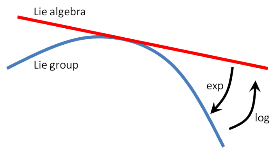
위 그림은 Lie 군과 그 접평면에 해당하는 Lie 대수의 관계를 보여주며, 서로 exponential과 logarithm 매핑을 통해 변환될 수 있음을 그리고 있다. 예를 들어 위에서 도출된 $\dot{\mathbf{R}}(t)=\hat{\mathbf{a}}\mathbf{R}(t)$은 일종의 미분 방정식으로 볼 수 있다. 해당 형태의 미분 방정식의 해는 exponential로 나타나며, 다음과 같다.

이것이 Lie 대수의 exponential 매핑이며, Lie 대수를 Lie 군으로 변환한다. 또한 양변에 로그를 취하면 Lie 군에서 Lie 대수로의 매핑을 구할 수 있으며, 이를 logarithm 매핑이라고 한다.

3. Lie Algebra의 특성

어떤 Lie 군에 대응되는 Lie algebra는 vector space $\mathcal{V}$, 어떤 field $\mathcal{F}$, Lie bracket이라고 불리는 이항연산자 $[\cdot, \cdot]$을 포함하고 있으며, 아래와 같은 특성을 갖는다.

• Closure: $[\mathbf{X}, \mathbf{Y}] \in \mathcal{V}$
• Bilinearity: $[a\mathbf{X}+b\mathbf{Y}, \mathbf{Z}]=a[\mathbf{X}, \mathbf{Z}]+b[\mathbf{Y}, \mathbf{Z}]$, $[\mathbf{Z}, a\mathbf{X}+b\mathbf{Y}]=a[\mathbf{Z}, \mathbf{X}] +b[\mathbf{Z}, \mathbf{Y}]$
• Alternating: $[\mathbf{X}, \mathbf{X}]=0$
• Jacobi identity: $[\mathbf{X},[\mathbf{Y}, \mathbf{Z}]]+[\mathbf{Y},[\mathbf{Z},\mathbf{X}]]+[\mathbf{Z},[\mathbf{X}, \mathbf{Y}]]=0$

Lie 군($SO(3), SE(3)$)은 그에 대응하는 Lie 대수($so(3), se(3)$)를 가지고 있으며, 각각은 다음과 같이 정의가 가능하다.

3.1. SO(3): Rotation

$SO(3)$군에 대한 Lie 대수는 다음과 같이 정의할 수 있다.

• Vector space: $so(3)=\{ \mathbf{\Phi} = \mathbf{\phi}^\wedge \in \mathcal{R}^{3 \times 3} | \mathbf{\phi} \in \mathcal{R}^3 \}$
• Field: $\mathcal{R}$
• Lie bracket: $[\mathbf{\Phi}_1, \mathbf{\Phi}_2] = \mathbf{\Phi}_1\mathbf{\Phi}_2-\mathbf{\Phi}_2\mathbf{\Phi}_1$

여기서 $\mathbf{\phi}^\wedge$는 위에서 보았듯이 다음과 같은 skew-symmetric 행렬이다.

Skew-symmetric의 성질을 이용하면 위의 정의가 Lie 특성 네 가지를 만족함을 알 수 있다. 예를 들어 closure는 다음과 같다.

여기서 $\mathbf{\phi}_1^\wedge\mathbf{\phi}_2^\wedge \in \mathcal{R}^3$이며, 추가적으로 $[\mathbf{\Phi}, \mathbf{\Phi}]=0$이다.

위에서도 보았듯이 $\mathbf{\phi}$는 각속도에 대응한다.

3.2. SE(3): Pose

$SE(3)$군에 대한 Lie 대수도 위와 비슷하게 정의할 수 있다.

• Vector space: $se(3)=\{ \mathbf{\Xi} = \mathbf{\xi}^\wedge \in \mathcal{R}^{4 \times 4} | \mathbf{\xi} \in \mathcal{R}^6 \}$
• Field: $\mathcal{R}$
• Lie bracket: $[\mathbf{\Xi}_1, \mathbf{\Xi}_2] = \mathbf{\Xi}_1\mathbf{\Xi}_2-\mathbf{\Xi}_2\mathbf{\Xi}_1$

$\mathbf{\xi}^\wedge$는 다음과 같이 정의하며, 여기서는 $^\wedge$연산자가 skew-symmetric 연산은 아니지만 $SO(3)$와의 통일성을 위해 그대로 사용한다.

여기서 $\mathbf{\phi}^\wedge$는 회전행렬 $\mathbf{R}$에 해당하는 Lie 대수이며, $\mathbf{\rho}$는 translation에 해당하고, $\mathbf{\phi}$를 twist라고 부르기도 한다.

$\phi$가 각속도에 대응하듯, $\rho$ 또한 선속도에 대응한다. $SO(3)$에서와 비슷하게 $\mathbf{T}\mathbf{T}^{-1}=\mathbf{I}$이고, 위처럼 $\dot\mathbf{T}\mathbf{T}^{-1}=\mathbf{\xi}^\wedge$의 결과가 나온다. 이를 풀어쓰면 다음과 같다.

여기서 $\rho=\dot\mathbf{t}-\dot\mathbf{R}\mathbf{R}^T\mathbf{t}=\dot\mathbf{t}+\mathbf{\phi}^\wedge(-\mathbf{t})$인데, 이는 translation 속도에 각속도로 인한 선속도를 합한 것이며, 최종적인 선속도가 된다.

4. 지수 및 로그 매핑

이제 Lie 군과 Lie 대수를 서로 변환하는 exponential(지수 매핑, Lie 대수에서 Lie 군), logarithm(로그 매핑, Lie 군에서 Lie 대수) 매핑을 알아보자.

여기서 사용될 지수와 로그에 대한 Taylor 전개는 다음과 같다.

4.1. SO(3): Rotation

$SO(3)$군부터 시작하면, 위에서 보았듯이 지수 매핑을 통해 $so(3) \rightarrow SO(3)$의 변환이 가능하다. 다만, 지수 매핑에서 자연상수 $e$의 지수에 있는 항은 일반적인 스칼라 값이 아닌 행렬이므로 지수를 계산하기 위하여 Taylor 전개를 이용하게 된다.

Lie 대수 $\mathbf{\phi}^{\wedge}$에 대해서 $\mathbf{\phi}=|\mathbf{\phi}|\mathbf{a}$인 단위 벡터 $\mathbf{a}$를 찾을 수 있고, $\mathbf{\phi}^{\wedge}=|\mathbf{\phi}|\mathbf{a}^{\wedge}$로 둘 수 있다. 이를 지수 매핑에 적용하여 Taylor 전개를 적용하면 다음과 같다.

Taylor 전개를 정리하는 과정에서 $\mathbf{a}^{\wedge}\mathbf{a}^{\wedge} = -\mathbf{I} + \mathbf{a}\mathbf{a}^T$, $\mathbf{a}^{\wedge}\mathbf{a}^{\wedge}\mathbf{a}^{\wedge}=-\mathbf{a}^{\wedge}$의 관계가 사용되었으며, 3번째 줄에서 4번째 줄로 넘어가는 과정에서는 다음과 같은 삼각함수의 Taylor 전개가 사용되었다.

위의 결과식은 로드리게스 식과 일치하며, 즉, $exp(\mathbf{\phi}^{\wedge}) = exp(|\mathbf{\phi}|\mathbf{a}^{\wedge})$은 $\mathbf{a}$을 축으로 $|\mathbf{\phi}|$ 만큼 회전하는 회전행렬과 같다. 따라서 Lie 대수 $\mathbf{\phi}^{\wedge}$를 지수함수를 통해 Lie 군인 $SO(3)$에 속하는 회전행렬로 매핑할 수 있다.

추가적으로 회전행렬을 $\mathbf{C}$이 주어졌을 때, 이에 대응하는 Lie 대수 $\mathbf{\phi}^{\wedge}$를 찾기 위하여 다음과 같은 로그 매핑을 수행해야 한다($^\vee$연산은 $^\wedge$의 역).

하지만 이전 글에서 회전행렬을 이용해 회전축과 각도를 구하는 방법을 유도하였기 때문에 굳이 지수 매핑처럼 Taylor 전개를 수행할 필요는 없다. 회전축 $\mathbf{a}$는 회전행렬 $\mathbf{C}$의 고유값 1에 대응하는 고유벡터임이며, 회전 각도는 다음과 같다.

뒤에 $2 \pi m$이 추가된 이유는 360도 단위로 회전하면 다시 제자리로 돌아오기 때문이며, 이로부터 매핑들이 1대1 매핑은 아니라는 것을 알 수 있지만, 회전 각도를 $0$에서 $2\pi$로 제한하면 1대1 매핑이 된다.

이렇게 구한 회전 행렬은 $SO(3)$군에 속하는데 Jacobi's formula(아래 식에서 2번째 term에서 3번째로 넘어갈 때 사용됨)를 이용하여 $det(\mathbf{C})=det(exp(\phi^\wedge))=exp(tr(\phi^\wedge))=exp(0)=1$등 $SO(3)$군의 성질을 만족함을 보일 수도 있다.

4.2. SE(3): Pose

Pose를 나타내는 $SE(3)$에서도 비슷한 형태로 지수 매핑($se(3) \rightarrow SE(3)$)과 로그 매핑($SE(3) \rightarrow se(3)$)이 계산될 수 있다. 먼저, 지수 매핑의 경우 다음과 같다 (아래 식은 $se(3)$의 정의를 이용하여 전개해보면 알 수 있음).

여기서 $\mathbf{r}, \mathbf{J}$는 다음과 같다.

앞에서 이미 $\mathbf{C} \leftrightarrow \phi^\wedge$ 사이의 변환 방법을 살펴보았기 때문에 여기서는 $\mathbf{r} \leftrightarrow \rho$의 관계만 살펴보며, 위의 전개에서 $\mathbf{r}=\mathbf{J}\rho$(지수 매핑에 사용), $\rho=\mathbf{J}^{-1}\mathbf{r}$(로그 매핑에 사용)의 관계가 있음을 알 수 있다.6

$\mathbf{J}$를 더 자세히 전개해보면 다음과 같다.

위의 식은 로드리게스 식과 비슷하지만 일치하지는 않는 것에 주의해야한다. 위의 식을 이용하면 $\mathbf{J}^{-1}$를 다음과 같이 구할 수 있다.

추가적으로 $\mathbf{J}$와 관련하여 유용한 몇 가지 식을 더 유도해보면 다음과 같다.

이때, $\mathbf{J}\mathbf{J}^T$은 양의 정부호행렬이다. 우선 $|\phi|=0$일 경우에는 $\mathbf{J}\mathbf{J}^T=\mathbf{I}$이 되어 양의 정부호행렬이 되고, $|\phi|\ne 0$일 경우에는 다음과 같이 보일 수 있다.

여기서 $(\mathbf{a}^T\mathbf{x})^T(\mathbf{a}^T\mathbf{x})$ 형태의 term은 norm을 계산하는 식이므로 $\mathbf{a},\mathbf{x}$가 수직일 경우에만 0이 된다.

그리고 $\mathbf{J}$와 $\mathbf{C}$사이에는 다음과 같은 관계가 존재한다.

특히 여기서 사용된 $\mathbf{J}$는 $SO(3)$의 (left) Jacobian이라고 한다.

Figure 2. Lie 대수, $se(3)$에서 각 원소의 의미(translation과 rotation)

5. 미분

일반적인 스칼라 값에 대해서 지수 계산는 $exp(a)exp(b)=exp(a+b)$와 같이 계산된다. 하지만 Lie 대수의 지수매핑에서는 지수에 행렬이 사용되기 때문에 이러한 식이 성립하지 않는다. 그 대신 Baker-Campbll-Hausdorff(BCH) 식에 의해 다음과 같이 지수 계산을 수행 할 수 있다.

위에서 사용된 $[\cdot,\cdot]$연산은 Lie bracket이다. 하지만 위의 식을 모두 계산하기는 매우 어렵기 때문에 보통 근사식을 사용하게 된다.

5.1. SO(3): Rotation

위의 BCH식을 이용하여 $\mathbf{C_1}=exp(\phi_1^\wedge), \mathbf{C_2}=exp(\phi_2^\wedge)$이라고 하면 다음과 같이 두 $SO(3)$의 합성에 대한 식을 계산할 수 있다.

여기서 $\mathbf{J}_l$는 SO(3)에 대한 left Jacobian, $\mathbf{J}_r$는 right Jacobian이라고 한다. 첫번째 경우를 예를 들면, $\mathbf{C_2}$에 아주 작은 회전 $\mathbf{C_1}$이 추가되었을 경우 그에 해당하는 Lie 대수는 $\mathbf{J}_l(\phi_2)\phi_1 + \phi_2$로 주어지며 $\mathbf{C_2}$에 대응하는 Lie 대수 $\phi_2$에 $\mathbf{J}_l(\phi_2)\phi_1$가 곱해진 경우이다(미소 변화에 미분값(Jacobian)이 곱해진 형태). $\mathbf{J}_l$와 그 역행렬은 위에서 구하였으며, $\mathbf{J}_r(\phi)=\mathbf{J}_l(-\phi)$, $\mathbf{J}_l(\phi)=\mathbf{C}\mathbf{J}_r(\phi)$의 관계가 있다($\mathbf{C}=exp(\phi^\wedge)$).

케이스가 두 가지로 구분되므로, 미소 변화가 왼쪽에 곱해지는지, 오른쪽에 곱해지는지 구분하여 사용하여야 한다. 최적화 등의 문제를 Lie 대수를 통해 해결할 경우 Lie 대수에 직접 미소 변화가 더해지거나, 아니면 Lie 군에서 미소 변화가 곱해지는 경우가 있다($SO(3)$를 보면 덧셈에 대해 닫혀있지 않아 미소 변화를 적용하려면 곱해야 함). 왼쪽 경우만 살펴보면 다음과 같다.

이제 위의 결과를 이용하여 $SO(3)$에 대한 미분을 $so(3)$를 이용하여 수행해보자. 이러한 미분은 Gauss_Newton과 같은 gradient descent 기반 최적화 등에 사용될 수 있다. 가장 먼저 떠올릴 수 있는 방법은 다음과 같이 회전하는 점 $\mathbf{C}\mathbf{v}$에 대해 $\phi$로 직접 미분하는 방법이다($\mathbf{l}$은 $\phi$에 대한 미소 변화의 방향).

만약 $\mathbf{C}\mathbf{v}$가 어떤 scalar 함수(error 함수 등) 안에 있다면 다음과 같이 미분이 계산될 수 있다. 만약 그 함수가 $u(\mathbf{x})$이고, $\mathbf{x}=\mathbf{C}\mathbf{v}$라면 다음과 같다.

Gradient descent 기반 최적화에서 linearization한 지점이 $\mathbf{C}_{op}=exp(\phi_{op}^\wedge)$라고 하면 다음과 같이 최적화를 진행할 수 있다.

하지만 여기서 Jacobian $\mathbf{J}$는 복잡한 형태를 가지고 있기 때문에 계산이나 구현 등이 어려워질 수 있다.

이러한 문제를 해결하는 방법으로, 미소 회전 $\Delta \mathbf{C}=exp(\psi^\wedge)$로 두고 $\psi$에 대해 미분하는 섭동 모델 방법이 있다(왼쪽에 미소 회전을 곱하는 경우).

위의 결과에서는 $\mathbf{J}$가 나오지 않아 더 간단하게 계산이 가능하다.

Scalar 함수(error 함수 등)를 가정했을때, 최적화의 대상이 되는 cost function은 다음과 같다(가장 많이 사용되는 최소제곱문제의 형태).

위의 cost function은 여러개의 scalar 함수가 합쳐진 최소제곱문제 형태이다. $\mathbf{C}_{op}$를 선형화 지점에서의 회전행렬, 미소 회전행렬을 왼쪽에 곱하는 섭동모델을 $\mathbf{C} = exp(\psi^\wedge)\mathbf{C}_{op}$라고 했을 때, 각 scalar 함수는 다음과 같이 쓸 수 있다.

이제 $J$는 $\psi$에 대한 식으로 표현되었으며, 다음과 같이 쉽게 미분이 가능하다.

$J$가 최소가 되기 위하여 위의 미분값이 0이 되어야 하므로, 다음과 같다.

위의 식은 최적의 값인 $\psi^*$에 대한 선형 방정식이므로 쉽게 해결이 가능하며, 이를 이용하여 다음과 같이 업데이트가 가능하다.

5.2. SE(3): Pose

$SE(3)$의 경우에도 비슷한 형태를 갖는다. $\mathbf{T_1}=exp(\xi_1^\wedge), \mathbf{T_2}=exp(\xi_2^\wedge)$이라고 하면 다음과 같다.

여기서 각 Jacobian은 다음과 같이 정의된다.

이때, $\mathbf{\mathcal{T}}$를 $SE(3)$의 adjoint라고 하며, 이 또한 Lie 군의 성질을 만족하고, $\mathbf{\mathcal{T}}$에 대응하는 Lie 대수는 $\xi^\barwedge$이다.

이때, $SO(3)$와 비슷하게 $\mathbf{\mathcal{J}}_r(\xi)=\mathbf{\mathcal{J}}_l(-\xi)$, $\mathbf{\mathcal{J}}_l(\xi)=\mathbf{\mathcal{T}}\mathbf{\mathcal{J}}_r(\xi)$의 관계가 있으며, 미소 변화 적용 식 역시 같은 형태를 가지고 있다.

$SE(3)$군에서도 비슷한 방법으로 미분이 가능하다. 먼저 $^\odot$연산을 다음과 같이 정의한다.

$^\odot$연산은 $\xi^\wedge\mathbf{p}=\mathbf{p}^\odot\xi$, $(\mathbf{T}\mathbf{p})^\odot=\mathbf{T}\mathbf{p}^\odot\mathcal{T}^{-1}$ 등의 성질을 만족한다.

$^\odot$연산을 사용하면 $SE(3)$군에서의 미분을 다음과 같이 정의할 수 있다(바로 Lie 대수 $\xi$로 미분하는 경우와 왼쪽 섭동에 대한 Lie 대수 $\epsilon$으로 미분하는 경우).

Jacobian이 포함되지 않은 섭동 식으로 cost 함수를 미분해보면 다음과 같다.

여기서 최적의 $\epsilon$에서 cost 함수의 미분이 0이 되어야 한다.

여기서 우리는 Lie 대수를 최적화 등에 사용할 때의 장점을 알 수 있다. 많이 사용되는 Gauss-Newton 기반의 최적화를 살펴보면 미소 변화를 더하며 업데이트를 수행하고 그 과정을 반복하여 최적화를 진행한다. 하지만 $SO(3), SE(3)$등은 더하기에 닫혀있지 않으며, 여러 제약조건을 가지고 있다(정규 직교, 행렬식이 1 등). 이에 비해 Lie 대수는 더하기에 대해 닫혀있으며, 그 수치에 대한 제약조건이 없다(지수 매핑을 통해 언제나 제약조건을 만족하는 Lie 군으로 매핑할 수 있음).