개요
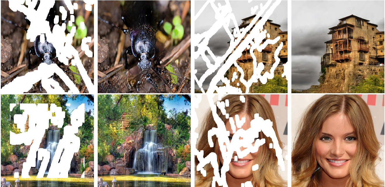
Image inpainting은 이미지의 빈 공간을 자연스럽고, 그럴듯 하게 채워넣는 것을 뜻한다.
이번 포스팅에서는 코드 위주로 풀어나가 보겠다.
튜토리얼에서 많이 사용하는 CIFAR10 데이터 셋과 기본 Autoencoder 모델을 사용하였다.
Code
아래의 깃허브에서 Tensorflow로 작성된 코드를 Pytorch로 재작성하였다.
https://github.com/ayulockin/deepimageinpainting
환경
- python 3.8.16
- numpy 1.24.3
- pytorch 2.1.0
- torchvision 0.16.0
- torchinfo 1.8.0
- Pillow 10.1.0
- tqdm 4.66.1
구현
1. Import Dependencies
from PIL import Image, ImageDraw
import numpy as np
import matplotlib.pyplot as plt
from tqdm import tqdm
import time

from IPython import display

import torch
from torch import nn, optim
from torch.utils.data import random_split, DataLoader, Dataset

from torchinfo import summary

import torchvision
import torchvision.transforms as transforms

from mpl_toolkits.axes_grid1 import ImageGrid

DEVICE = torch.device("mps") # M1 mac GPU setting
DEVICE
2. Set hyperparameters
SEED = 88
VAL_RATIO = 0.25

BATCH_SIZE = 32
EPOCHS = 50
LR = 0.00007

PRINT_FLUSH = True
3. Prepare DataLoader
class CustomDataset(Dataset):
    def __init__(self, data, transform = None):
        self.data = data
        self.transform = transform

    def __len__(self):
        return self.data.shape[0]

    def __getitem__(self, idx):
        img = self.data[idx]
        masked_img = self.__create_masked_img(img)

        if self.transform is not None:
            img = self.transform(img)
            masked_img = self.transform(masked_img)

        return masked_img, img

    def __create_masked_img(self, img):

        # Prepare mask
        mask_array = np.full((img.shape), 255, np.uint8)
        mask = Image.fromarray(mask_array)
        draw = ImageDraw.Draw(mask)

        for _ in range(np.random.randint(1, 10)):

            # Get random x locatioins to start line
            x1, x2 = np.random.randint(1, img.shape[1]), np.random.randint(1, img.shape[1])

            # Get random y locations to start line
            y1, y2 = np.random.randint(1, img.shape[0]), np.random.randint(1, img.shape[0])

            # Get random thickness of the line drawn
            thickness = np.random.randint(1, 3)

            # Draw black line on the white mask
            draw.line((x1, y1, x2, y2), fill = "black", width = thickness)

        masked_img = img.copy()
        masked_img[np.array(mask) == 0] = 255

        return masked_img
trainset = torchvision.datasets.CIFAR10(root = "./data", train = True, download = True)
testset = torchvision.datasets.CIFAR10(root = "./data", train = False, download = True)
train_subset, val_subset = random_split(trainset, [1 - VAL_RATIO, VAL_RATIO], generator = torch.Generator().manual_seed(SEED))
train_data = train_subset.dataset.data[train_subset.indices]
val_data = val_subset.dataset.data[val_subset.indices]
test_data = testset.datatransform = transforms.Compose([
transforms.ToTensor(),
])
train_dataset = CustomDataset(data = train_data, transform = transform)
val_dataset = CustomDataset(data = val_data, transform = transform)
test_dataset = CustomDataset(data = test_data, transform = transform)
train_loader = DataLoader(train_dataset, batch_size = BATCH_SIZE, shuffle = True)
val_loader = DataLoader(val_dataset, batch_size = BATCH_SIZE, shuffle = True)
test_loader = DataLoader(test_dataset, batch_size = BATCH_SIZE, shuffle = False)torchvision의 CIFAR10 데이터는 Image classification에 적합한 데이터 이므로 Image inpainting이라는 목적에 맞게 데이터셋을 새로 구성해야 했기 때문에 CustomDataset을 정의했고 이후 재구성한 dataset으로 dataloader를 구성했다.
sample_imgs, sample_masked_imgs = next(iter(train_loader))

sample_imgs_batch = [None] * (len(sample_masked_imgs) + len(sample_imgs))
sample_imgs_batch[::2] = sample_imgs.permute(0, 2, 3, 1)
sample_imgs_batch[1::2] = sample_masked_imgs.permute(0, 2, 3, 1)

fig = plt.figure(figsize = (16., 8.))
grid = ImageGrid(fig, 111, nrows_ncols = (4, 8), axes_pad = 0.3)

for ax, img in zip(grid, sample_imgs_batch):
    ax.imshow(img)

plt.show()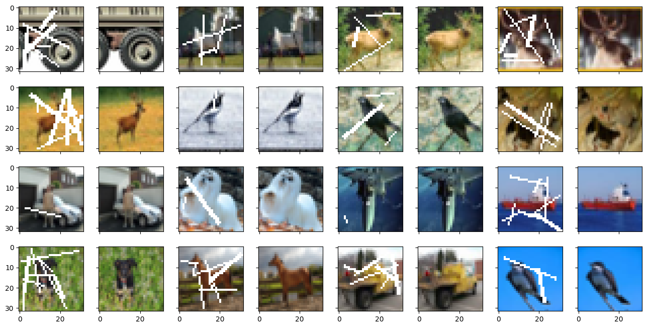
train_loader에서 임의로 하나의 배치를 뽑아 시각화 해보니 의도한대로 데이터 셋이 구성된 것을 확인할 수 있었다.
4. Model
class BasicConv(nn.Module):
    def __init__(self, in_channels, out_channels, kernel_size = 3, padding = 1, last = False):
        super().__init__()

        self.conv = nn.Sequential(
            nn.Conv2d(in_channels, out_channels, kernel_size = kernel_size, padding = padding, bias = False),
            nn.BatchNorm2d(out_channels),
        )
        self.activation = nn.Sigmoid() if last else nn.ReLU(inplace = True)

        for m in self.modules():
            if isinstance(m, nn.Conv2d):
                nn.init.kaiming_normal_(m.weight, mode = "fan_out", nonlinearity = "relu")

    def forward(self, x):
        x = self.conv(x)
        x = self.activation(x)
        return x

class DownConvBlock(nn.Module):
    def __init__(self, in_channels, out_channels):
        super().__init__()

        self.conv = nn.Sequential(
            BasicConv(in_channels, out_channels),
            BasicConv(out_channels, out_channels)
        )
        self.pool = nn.MaxPool2d(2)

        for m in self.modules():
            if isinstance(m, nn.Conv2d):
                nn.init.kaiming_normal_(m.weight, mode = "fan_out", nonlinearity = "relu")

    def forward(self, x):
        conv = self.conv(x)
        pool = self.pool(conv)
        return conv, pool

class UpConvBlock(nn.Module):
    def __init__(self, in_channels, inner_channels, out_channels):
        super().__init__()

        self.conv = nn.Sequential(
            BasicConv(in_channels, inner_channels),
            BasicConv(inner_channels, inner_channels)
        )
        self.up = nn.Sequential(
            nn.ConvTranspose2d(inner_channels, out_channels, kernel_size = 2, stride = 2, bias = False),
            nn.BatchNorm2d(out_channels),
            nn.ReLU(inplace = True),
        )

        for m in self.modules():
            if isinstance(m, nn.Conv2d) or isinstance(m, nn.ConvTranspose2d):
                nn.init.kaiming_normal_(m.weight, mode = "fan_out", nonlinearity = "relu")

    def forward(self, x):
        x = self.conv(x)
        x = self.up(x)
        return x

class AutoEncoder(nn.Module):
    def __init__(self, in_channels = 3):
        super().__init__()

        self.down1 = DownConvBlock(in_channels, 32)
        self.down2 = DownConvBlock(32, 64)
        self.down3 = DownConvBlock(64, 128)
        self.down4 = DownConvBlock(128, 256)

        self.up1 = UpConvBlock(256, 512, 256)
        self.up2 = UpConvBlock(512, 256, 128)
        self.up3 = UpConvBlock(256, 128, 64)
        self.up4 = UpConvBlock(128, 64, 32)

        self.last_conv = nn.Sequential(
            BasicConv(64, 32),
            BasicConv(32, 32),
            BasicConv(32, 3, last = True),
        )

        for m in self.modules():
            if isinstance(m, nn.Conv2d) or isinstance(m, nn.ConvTranspose2d):
                nn.init.kaiming_normal_(m.weight, mode = "fan_out", nonlinearity = "relu")

    def forward(self, x):
        feature1, x = self.down1(x)
        feature2, x = self.down2(x)
        feature3, x = self.down3(x)
        feature4, x = self.down4(x)

        x = self.up1(x)
        x = self.up2(torch.cat([x, feature4], dim = 1))
        x = self.up3(torch.cat([x, feature3], dim = 1))
        x = self.up4(torch.cat([x, feature2], dim = 1))

        x = self.last_conv(torch.concat([x, feature1], dim = 1))

        return x
참고한 링크의 Tensorflow로 작성된 모델에서 batch normalization과 weight initialization을 추가했다.
model = AutoEncoder()
summary(model, input_size = (2, 3, 32, 32))
===============================================================================================
Layer (type:depth-idx) Output Shape Param #
===============================================================================================
AutoEncoder [2, 3, 32, 32] --
├─DownConvBlock: 1-1 [2, 32, 32, 32] --
│ └─Sequential: 2-1 [2, 32, 32, 32] --
│ │ └─BasicConv: 3-1 [2, 32, 32, 32] 928
│ │ └─BasicConv: 3-2 [2, 32, 32, 32] 9,280
│ └─MaxPool2d: 2-2 [2, 32, 16, 16] --
├─DownConvBlock: 1-2 [2, 64, 16, 16] --
│ └─Sequential: 2-3 [2, 64, 16, 16] --
│ │ └─BasicConv: 3-3 [2, 64, 16, 16] 18,560
│ │ └─BasicConv: 3-4 [2, 64, 16, 16] 36,992
│ └─MaxPool2d: 2-4 [2, 64, 8, 8] --
├─DownConvBlock: 1-3 [2, 128, 8, 8] --
│ └─Sequential: 2-5 [2, 128, 8, 8] --
│ │ └─BasicConv: 3-5 [2, 128, 8, 8] 73,984
│ │ └─BasicConv: 3-6 [2, 128, 8, 8] 147,712
│ └─MaxPool2d: 2-6 [2, 128, 4, 4] --
├─DownConvBlock: 1-4 [2, 256, 4, 4] --
│ └─Sequential: 2-7 [2, 256, 4, 4] --
│ │ └─BasicConv: 3-7 [2, 256, 4, 4] 295,424
│ │ └─BasicConv: 3-8 [2, 256, 4, 4] 590,336
│ └─MaxPool2d: 2-8 [2, 256, 2, 2] --
├─UpConvBlock: 1-5 [2, 256, 4, 4] --
│ └─Sequential: 2-9 [2, 512, 2, 2] --
│ │ └─BasicConv: 3-9 [2, 512, 2, 2] 1,180,672
│ │ └─BasicConv: 3-10 [2, 512, 2, 2] 2,360,320
│ └─Sequential: 2-10 [2, 256, 4, 4] --
│ │ └─ConvTranspose2d: 3-11 [2, 256, 4, 4] 524,288
│ │ └─BatchNorm2d: 3-12 [2, 256, 4, 4] 512
│ │ └─ReLU: 3-13 [2, 256, 4, 4] --
├─UpConvBlock: 1-6 [2, 128, 8, 8] --
│ └─Sequential: 2-11 [2, 256, 4, 4] --
│ │ └─BasicConv: 3-14 [2, 256, 4, 4] 1,180,160
│ │ └─BasicConv: 3-15 [2, 256, 4, 4] 590,336
│ └─Sequential: 2-12 [2, 128, 8, 8] --
│ │ └─ConvTranspose2d: 3-16 [2, 128, 8, 8] 131,072
│ │ └─BatchNorm2d: 3-17 [2, 128, 8, 8] 256
│ │ └─ReLU: 3-18 [2, 128, 8, 8] --
├─UpConvBlock: 1-7 [2, 64, 16, 16] --
│ └─Sequential: 2-13 [2, 128, 8, 8] --
│ │ └─BasicConv: 3-19 [2, 128, 8, 8] 295,168
│ │ └─BasicConv: 3-20 [2, 128, 8, 8] 147,712
│ └─Sequential: 2-14 [2, 64, 16, 16] --
│ │ └─ConvTranspose2d: 3-21 [2, 64, 16, 16] 32,768
│ │ └─BatchNorm2d: 3-22 [2, 64, 16, 16] 128
│ │ └─ReLU: 3-23 [2, 64, 16, 16] --
├─UpConvBlock: 1-8 [2, 32, 32, 32] --
│ └─Sequential: 2-15 [2, 64, 16, 16] --
│ │ └─BasicConv: 3-24 [2, 64, 16, 16] 73,856
│ │ └─BasicConv: 3-25 [2, 64, 16, 16] 36,992
│ └─Sequential: 2-16 [2, 32, 32, 32] --
│ │ └─ConvTranspose2d: 3-26 [2, 32, 32, 32] 8,192
│ │ └─BatchNorm2d: 3-27 [2, 32, 32, 32] 64
│ │ └─ReLU: 3-28 [2, 32, 32, 32] --
├─Sequential: 1-9 [2, 3, 32, 32] --
│ └─BasicConv: 2-17 [2, 32, 32, 32] --
│ │ └─Sequential: 3-29 [2, 32, 32, 32] 18,496
│ │ └─ReLU: 3-30 [2, 32, 32, 32] --
│ └─BasicConv: 2-18 [2, 32, 32, 32] --
│ │ └─Sequential: 3-31 [2, 32, 32, 32] 9,280
│ │ └─ReLU: 3-32 [2, 32, 32, 32] --
│ └─BasicConv: 2-19 [2, 3, 32, 32] --
│ │ └─Sequential: 3-33 [2, 3, 32, 32] 870
│ │ └─Sigmoid: 3-34 [2, 3, 32, 32] --
===============================================================================================
Total params: 7,764,358
Trainable params: 7,764,358
Non-trainable params: 0
Total mult-adds (M): 429.27
===============================================================================================
Input size (MB): 0.02
Forward/backward pass size (MB): 10.06
Params size (MB): 31.06
Estimated Total Size (MB): 41.14
===============================================================================================약 776만 개의 파라미터를 갖는 Autoencoder 모델임을 확인할 수 있다.
5. Train
# Metric
def dice_coef(y_true, y_pred):
    y_true_f = torch.flatten(y_true)
    y_pred_f = torch.flatten(y_pred)
    intersection = torch.sum(y_true_f * y_pred_f)
return (2. * intersection) / (torch.sum(y_true_f + y_pred_f))- Dice coefficient (다이스 계수)
두 집합간의 유사도를 측정하는데 사용된다.
컴퓨터 비전에서는 픽셀단위로 결과값을 봐야 하는 segmentation task에서 주로 이용하는 평가지표 이다.
image inpainting에서도 input 이미지와 모델이 예측한 이미지의 유사도를 측정하기 위해 사용할 수 있다.
두 집합이 0 ~ 1 의 값으로 구성되어 있다면 1 에 가까울 수록 두 집합이 유사하다고 해석할 수 있다.- 두 집합의 원소가 이진수로만 이루어져 있다면 % 를 이용한 해석이 가능하다.
ex)dice_coef = 0.8일 때, 두 집합은 80 % 정도의 유사도를 가진다. 라고 해석 가능. - 두 집합의 원소가 이진수가 아닌 0 ~ 1 사이의 값이라면 % 를 이용한 해석은 적절하지 않다.
상대적인 비교를 통해 어떤 두 집합이 다른 두 집합보다 유사도가 높은지 알 수 있다.
- 두 집합의 원소가 이진수로만 이루어져 있다면 % 를 이용한 해석이 가능하다.
class EarlyStopping:
    def __init__(self, patience = 5, thresh = 0.0, mode = "min", verbose = True):
        self.early_stop = False
        self.patience = patience
        self.verbose = verbose
        self.mode = mode
        self.thresh = thresh

        self.counter = 0
        self.best_score = np.Inf if mode == "min" else 0 if mode == "max" else AssertionError

    def step(self, score):
        if self.mode == "min":
            if score < (self.best_score - self.thresh):
                self.counter = 0
                self.best_score = score
            else:
                self.counter += 1
                if self.verbose:
                    print(f"[EarlyStopping] (Patience) {self.counter}/{self.patience}. "\
                          f"Best score: {self.best_score:.5f}"\
                          f", Current: {score:.5f}", flush = PRINT_FLUSH)


        elif self.mode == "max":
            if score > (self.best_score + self.thresh):
                self.counter = 0
                self.best_score = score
                if self.verbose:
                    print(f"[EarlyStopping] (Patience) {self.counter}/{self.patience}. "\
                          f"Best score: {self.best_score:.5f}"\
                          f", Current: {score:.5f}", flush = PRINT_FLUSH)

        if self.counter >= self.patience:
            if self.verbose:
                print(f"[EarlyStop Triggered] Best Score: {self.best_score:.5f}", flush = PRINT_FLUSH)

            #Early stop
            self.early_stop = True
criterion = nn.L1Loss()
metric = dice_coefEarly Stopping, criterion, metric을 정의해준다.
criterion은 각 픽셀값의 차이를 비교하기 위해 MAE를 사용하였다. (MSE는 MAE보다 오차에 민감하고 경계 부분에서 작은 차이도 크게 반영되기 때문에, 경계가 부드럽게 처리될 수 있고 이는 이미지를 흐릿하게 만들 수도 있음.)
metric은 이전 셀에서 정의한 다이스 계수를 사용하였다.
def loss_epoch(model, DL, criterion, metric, optimizer = None):
    N = len(DL.dataset) # the number of data
    r_loss = 0; r_score = 0
    for x_batch, y_batch in tqdm(DL, leave=False):

        x_batch, y_batch = x_batch.to(DEVICE), y_batch.to(DEVICE)

        # inference
        y_pred = model(x_batch)

        # Loss
        loss = criterion(y_pred, y_batch)

        # update
        if optimizer is not None:
            optimizer.zero_grad() # gradient 누적을 막기 위한 초기화
            loss.backward() # backpropagation
            optimizer.step() # weight update

        # loss accumulation
        loss_b = loss.item() * x_batch.shape[0]
        r_loss += loss_b # running loss

        # metric
        score_b = metric(y_batch, y_pred).item() * x_batch.shape[0]
        r_score += score_b

    loss_e = r_loss / N
    score_e = r_score / N

    return loss_e, score_e
def vis(model, masked_img, img):
masked_img = masked_img.to(DEVICE)
prediction = model(masked_img)
prediction = prediction.detach()
masked_img = masked_img[0].to("cpu")
prediction = prediction[0].to("cpu")
img = img[0].to("cpu")
masked_img = torch.permute(masked_img, [1, 2, 0])
prediction = torch.permute(prediction, [1, 2, 0])
img = torch.permute(img, [1, 2, 0])
display_list = [masked_img, img, prediction]
title = ["Input image", "Original image","Predicted image"]
length = len(display_list)
plt.figure(figsize = (15, 15))
for i in range(length):
plt.subplot(1, length, i + 1)
plt.title(title[i])
plt.imshow(display_list[i])
plt.axis("off")
plt.show()def draw_history(train_loss_list, val_loss_list, title):
assert len(train_loss_list) == len(val_loss_list)
if len(train_loss_list) < 2:
return None
train_loss_x_list = np.arange(0, len(train_loss_list), 1)
val_loss_x_list = np.arange(0, len(val_loss_list), 1)
plt.figure(figsize = (20, 10))
plt.plot(train_loss_x_list, train_loss_list, label = f"train {title}")
plt.plot(val_loss_x_list, val_loss_list, label = f"val {title}")
plt.title(title)
plt.show()그 밖에 모델 학습 과정에서 epoch 단위로 루프를 돌며 모델 학습을 진행할 loss_epoch 를 정의하고,
학습 과정 및 결과 모니터링을 위해 vis, draw_history 를 정의하였다.
# Load model
model = AutoEncoder()
model.to(DEVICE)

# Load object for training
optimizer = optim.Adam(model.parameters(), lr = LR)
lr_scheduler = optim.lr_scheduler.ReduceLROnPlateau(optimizer, mode = "min", factor = 0.1, patience = 10, cooldown = 3)
early_stopping = EarlyStopping(patience = 30, thresh = 0, mode = "min")

loss_history = {"train": [], "val" : []}
score_history = {"train": [], "val" : []}

best_loss = np.Inf; train_loss = np.Inf; val_loss = np.Inf
best_score = 0; train_score = 0; val_score = 0

# example image for visualization
example_masked_image, example_image = next(iter(val_loader))

# Model Training
for epoch in range(EPOCHS):
    display.clear_output(wait = True)
    vis(model, example_masked_image, example_image)

    epochs_start = time.time()
    current_lr = optimizer.param_groups[0]["lr"]
    print(f"Epoch: {epoch + 1}, current_LR = {current_lr}", flush = PRINT_FLUSH)
    print(f"Best val loss: {round(best_loss, 5)}, Best val score: {round(best_score, 5)}")
    print(f"train loss: {round(train_loss, 5)}, val loss: {round(val_loss, 5)}", flush = PRINT_FLUSH)
    print(f"train score: {round(train_score, 5)}, val score: {round(val_score, 5)} \n", flush = PRINT_FLUSH)

    draw_history(loss_history["train"], loss_history["val"], title = "loss")
    draw_history(score_history["train"], score_history["val"], title = "disc_coef")

    # Train
    model.train()
    train_loss, train_score = loss_epoch(model, train_loader, criterion, metric, optimizer)
    loss_history["train"].append(train_loss)
    score_history["train"].append(train_score)

    # Validation
    model.eval()
    with torch.no_grad():
        val_loss, val_score = loss_epoch(model, val_loader, criterion, metric)
        loss_history["val"].append(val_loss)
        score_history["val"].append(val_score)

        if val_loss < best_loss:
            best_loss = val_loss
            best_score = val_score
            torch.save({
                "model" : model,
                "epoch" : epoch,
                "optimizer" : optimizer,
                "scheduler" : lr_scheduler,
            }, f"./runs/pytorch_checkpoint/best.pt")

        print("-" * 20, flush = PRINT_FLUSH)

    lr_scheduler.step(val_loss)
    early_stopping.step(val_loss)
    if early_stopping.early_stop:
        break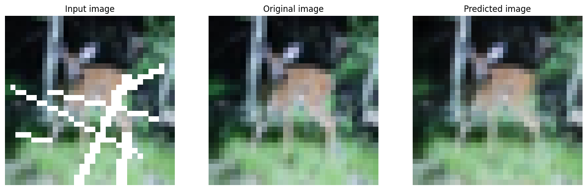
Epoch: 50, current_LR = 7e-05
Best val loss: 0.0137, Best val score: 0.60343
train loss: 0.01829, val loss: 0.01502
train score: 0.60456, val score: 0.60411 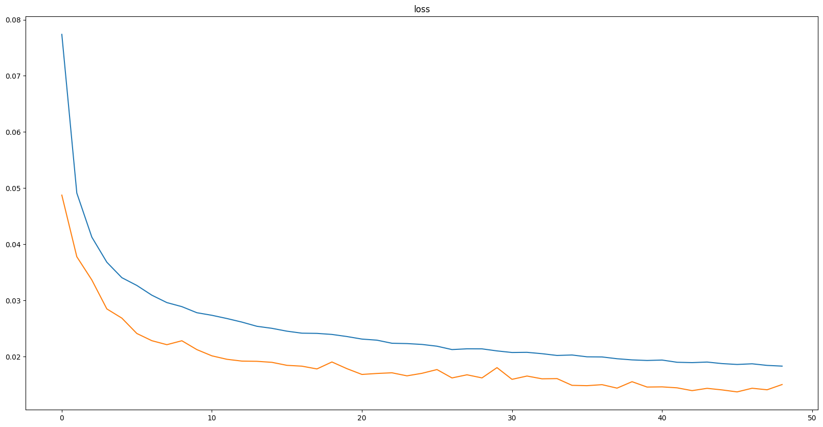
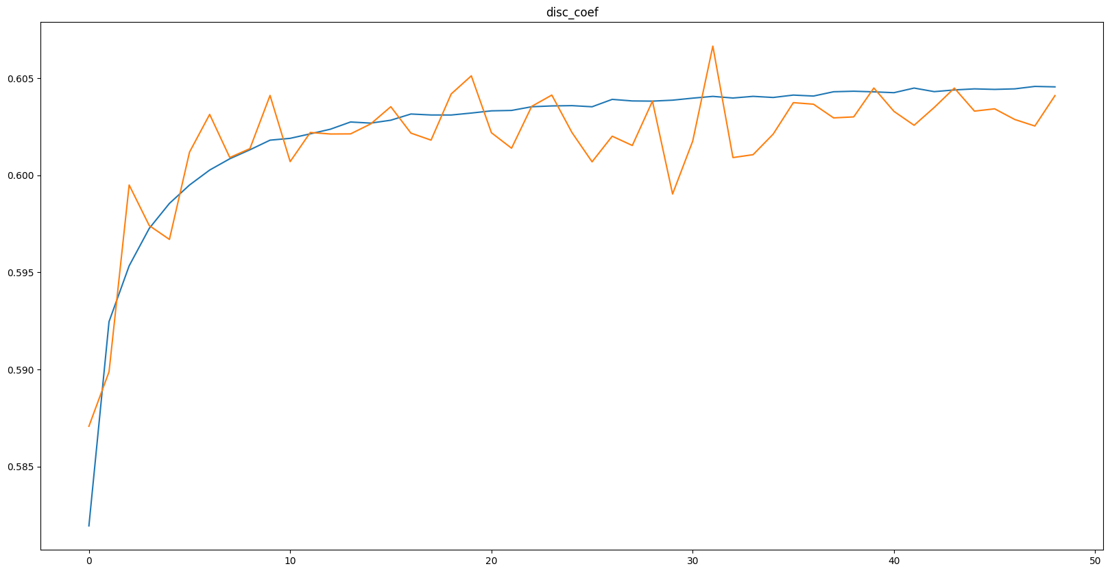
그래프에 주석을 안 달았는데 파란색이 train, 주황색이 val에 관한 지표이다.
과적합이 일어나지 않았고, loss 값이 어느정도 수렴하는 모습을 보인다.
학습이 끝난 모델(50 epochs) 이 만들어낸 샘플 이미지를 보니 어느정도 잘 inpainting 하는 것을 볼 수 있다.
6. Test
test_model = torch.load("./runs/pytorch_checkpoint/best.pt")
test_model['epoch'] # 45test_loss, test_score = loss_epoch(test_model["model"], test_loader, criterion, metric)
print(test_score) # 0.60653658485412645 번째 epoch를 거친 모델의 val_loss 값이 가장 낮았다.
해당 모델을 이용해 Test 데이터의 다이스 계수를 구해보면 약 0.6065 가 나온 것을 볼 수 있다.
test_masked_imgs, test_imgs = next(iter(test_loader))
for i in range(BATCH_SIZE):
    vis(test_model, test_masked_imgs[i].unsqueeze(0), test_imgs[i].unsqueeze(0))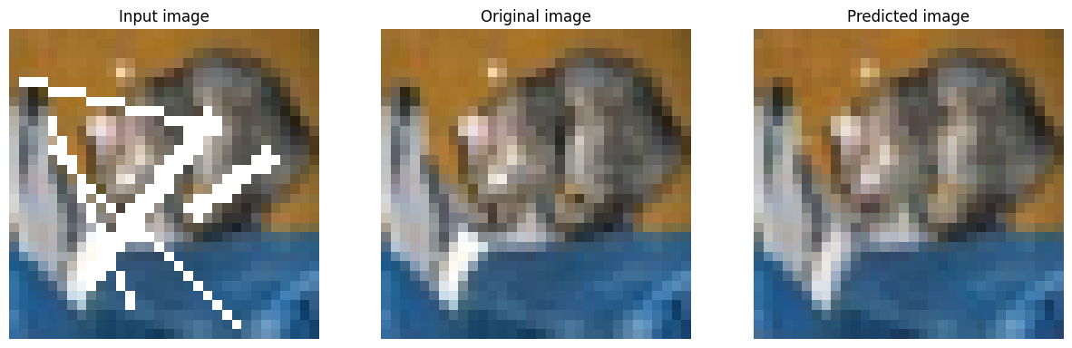
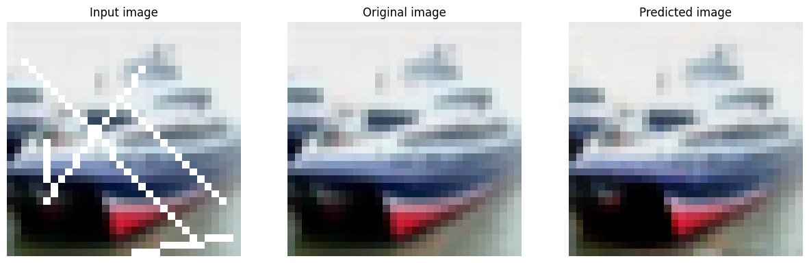
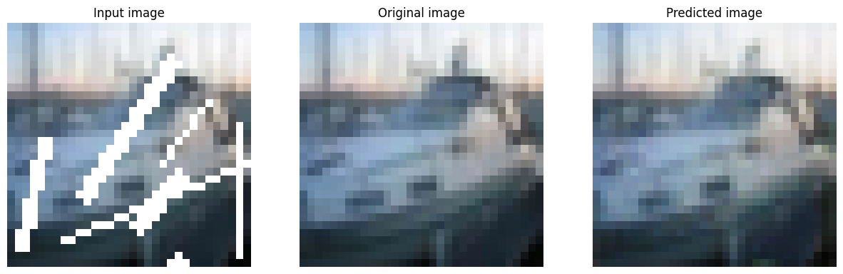
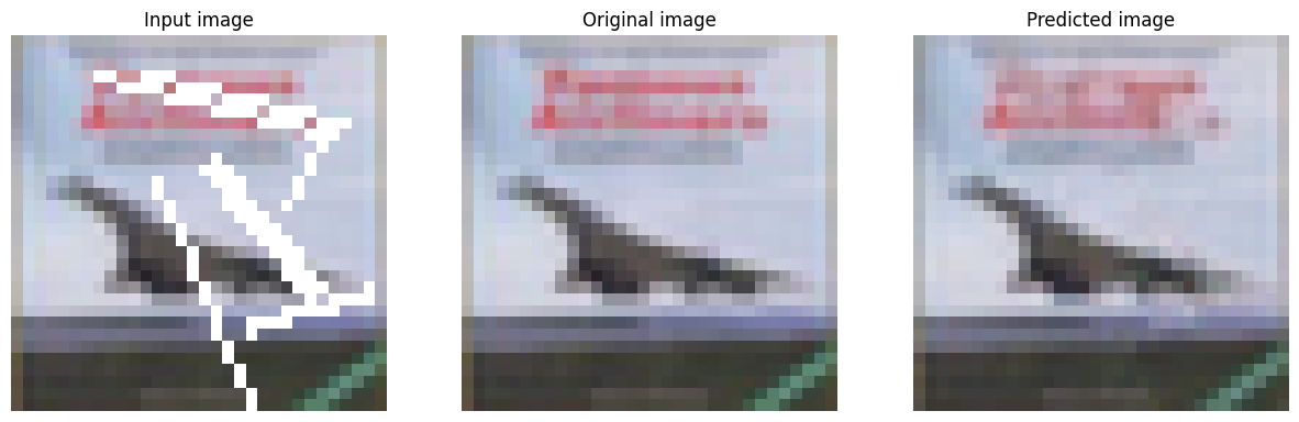
결과 이미지 일부를 보면 마찬가지로 어느정도 잘 inpainting 한 것을 볼 수 있다.
다만 CIFAR10 데이터셋 특성상 이미지가 너무 작아 (32 x 32) 육안으로 자연스럽게 느낄만큼 inpainting이 잘 된 것인지는 확인 할 수 없었다.