3장. 사이킷런을 타고 떠나는 머신 러닝 분류 모델 투어 -1
0

이 장에서 다룰 주제
- 강력하고 인기 있는 분류 알고리즘인 로지스틱 회귀, 서포트 벡터 머신, 결정 트리 소개하기
- 예제와 설명을 위해 사이킷런 머신 러닝 라이브러리 사용하기
- 선형 또는 비선형 결정 경계를 갖는 분류 알고리즘의 강점과 약점 설명하기
분류 알고리즘 선택
✨ 특정 문제에 알맞은 분류 알고리즘을 선택하려면 연습과 경험이 필요!!!
-
모든 경우에 뛰어난 성능을 낼 수 있는 분류 모델은 없다
-
최소한 몇 개의 학습 알고리즘 성능을 비교하고 해당 문제에 최선인 모델을 선택하는 것이 항상 권장
-
분류 모델의 예측 성능과 계산 성능은 학습에 사용하려는 데이터에 크게 의존한다
- 특성이나 샘플의 개수
- 데이터셋에 있는 잡음 데이터의 양
- 클래스가 선형적으로 구분되는지 아닌지에 따라
-
머신러닝 알고리즘을 훈련하기 위한 다섯 가지 주요 단계
- 특성을 선택하고 훈련 샘플을 모은다
- 성능 지표를 선택
- 분류 모델과 최적화 알고리즘을 선택
- 모델의 성능을 평가
- 알고리즘을 튜닝
사이킷럿 첫걸음: 퍼셉트론 훈련
from sklearn import datasets
import numpy as np
📍 데이터 불러오기
iris = datasets.load_iris()
x = iris.data[:, [2, 3]]
y = iris.target

print('클래스 레이블', np.unique(y))

~~>
클래스 레이블 [0 1 2]
💡 클래스 레이블
- Iris-setosa : 0
- Iris-versicolor : 1
- Iris-virginica : 2
✨ 사소한 실수를 피할 수 있고 작은 메모리 영역을 차지하므로 계산 성능을 향상기키기 때문에 정수 레이블을 사용
📍 데이터셋 분할
- 사이킷런 model_selection 모듈의 train_test_split 함수를 사용해서 x와 y 배열을 랜덤하게 나눈다
from sklearn.model_selection import train_test_split

x_train, x_test, y_train, y_test = train_test_split(x, y, test_size=0.3, random_state=1, stratify=y)

print('y의 레이블 카운트 : ', np.bincount(y))
print('y_train의 레이블 카운트 : ', np.bincount(y_train))
print('y_test의 레이블 카운트 : ', np.bincount(y_test))

~~>
y의 레이블 카운트 : [50 50 50]
y_train의 레이블 카운트 : [35 35 35]
y_test의 레이블 카운트 : [15 15 15]random_state=1을 통해 랜덤 시드를 고정
stratify=y를 통해 계층화 기능을 사용
💡 계층화란 데이터셋과 테스트 데이터셋의 클래스 레이블 비율을 입력 데이터셋과 동일하게 만드는 것
📍 표준화
- StandardScaler 클래스를 사용하여 특성을 표준화
from sklearn.preprocessing import StandardScaler

sc = StandardScaler()
sc.fit(x_train)
x_train_std = sc.trainsform(x_train)
x_test_std = sc.transform(x_test)- 특성 차원마다 샘플 평균과 표준 편차를 계산해 훈련 데이터셋을 표준화
- 훈련 데이터셋과 테스트 데이터셋의 샘플이 서로 같은 비율로 이동되도록 동일한 샘플 평균과 표준 편차를 사용하여 테스트 데이터셋을 표준화
from sklearn.linear_model import Perceptron

ppn = Perceptron(eta=0.1, random_state=1)
ppn.fit(x_train_std, y_train)
y_pred = ppn.predict(x_test_std)
print('잘못 분류된 샘플 개수 : %d' %(y_test != y_pred).sum()
~~>
잘못 분류된 샘플 개수 : 1- 45개의 샘플에서 한 개를 잘못 분류
- 테스트 데이터셋에 대한 분류 오차는 약
0.022또는2.2%(1/45)
from sklearn.metrics import accuracy_score

print('정확도 : %.3f' %accuracy_score(y_test, y_pred))
print('정확도 : %.3f' %ppn.score(x_test_std, y_test))

~~>
정확도 : 0.978
정확도 : 0.978
📍 시각화
- 퍼셉트론 모델의 결정경계 시각화를 통해 붓꽃 샘플을 잘 구분하는지 시각화
from matplotlib.colors import ListedColormap
import matplotlib.pyplot as plt

def plot_decision_regions(x, y, classifier, test_idx=None, resolution=0.02):
    # 마커와 컬러맵을 설정
    markers = ('s', 'x', 'o', '^', 'v')
    colors = ('red', 'blue', 'lightgreen', 'gray', 'cyan')
    cmap = ListedColormap(colors[:len(np.unique(y))])

    # 결정 경계 그리기
    x1_min, x1_max = x[:, 0].min() -1, x[:, 0].max() +1
    x2_min, x2_max = x[:, 1].min() -1, x[:, 1].max() +1
    xx1, xx2 = np.meshgrid(np.arange(x1_min, x1_max, resolution),
                          np.arange(x2_min, x2_max, resolution))
    z = classifier.predict(np.array([xx1.ravel(), xx2.ravel()]).T)
    z = z.reshape(xx1.shape)

    plt.contourf(xx1, xx2, z, alpha=0.3, cmap=cmap)
    plt.xlim(xx1.min(), xx1.max())
    plt.ylim(xx2.min(), xx2.max())

    for idx, cl in enumerate(np.unique(y)):
        plt.scatter(x=x[y == cl, 0], y=x[y == cl, 1],
                   alpha=0.8, c=colors[idx],
                   marker=markers[idx], label=cl,
                   edgecolor='black')

    # 테스트 샘플을 부각하여 그리기
    if test_idx:
        x_test, y_test = x[test_idx, :], y[test_idx]

        plt.scatter(x_test[:, 0], x_test[:, 1],
                   facecolors='none', edgecolor='black', alpha=1.0,
                   linewidth=1, marker='o',
                   s=100, label='test set')
x_combined_std = np.vstack((x_train_std, x_test_std))
y_combined = np.hstack((y_train, y_test))
plot_decision_regions(x=x_combined_std,
y=y_combined,
classifier=ppn,
test_idx=range(105, 150))
plt.xlabel('petal length [stanardized]')
plt.ylabel('petal width [stanardized]')
plt.legend(loc='upper left')
plt.tight_layout()
plt.show()
~~>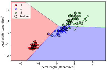
👉 선형 결정 경계로 완벽하게 분류되지 못하는 것을 볼 수 있다.
로지스틱 회귀를 사용한 클래스 확률 모델링
- 퍼셉트론 규칙의 큰 단점은 클래스가 선형적으로 구분되지 않을 때 수렴할 수 없다는 것
- 선형 이진 분류 문제에 더 강력한 다른 알고리즘인 로지스틱 회귀( logistic regression ) 을 사용하는것이 더 현명한 방법
- 로지스틱 회귀도 분류 모델
로지스틱 회귀
- 손쉽게 다중 클래스 설정으로 일반화할 수 있다.
- 다항 로지스틱 회귀 또는 소프트맥스 회귀라고 부른다
- 오즈비에 로그 함수( 로그 오즈 )를 취해 로짓( logit )함수를 정의
- 오즈는 특정 이벤트가 발생활 확률
- logit 함수는
0과1사이의 입력값을 받아 실수 범위 값으로 변환
- 이 함수를 로지스틱 시그모이드 함수 줄여서 시그모이드 함수라고 한다
📍 시그모이드 함수의 모습
def sigmoid(z):
    return 1.0 / (1.0 + np.exp(-z))

z = np.arange(-7, 7, 0.1)
phi_z = sigmoid(z)
plt.plot(z, phi_z)
plt.axvline(0.0, color='k')
plt.ylim(-0.1, 1.1)
plt.xlabel('z')
plt.ylabel('$\phi (z)$')

# y축의 눈금과 격자선
plt.yticks([0.0, 0.5, 1.0])
ax = plt.gca()
ax.yaxis.grid(True)
plt.tight_layout()

plt.show()

~~>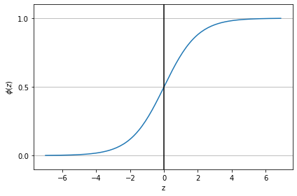
- 실수 입력 값을
[0, 1]사이의 값으로 변환 - 중간은
0.5
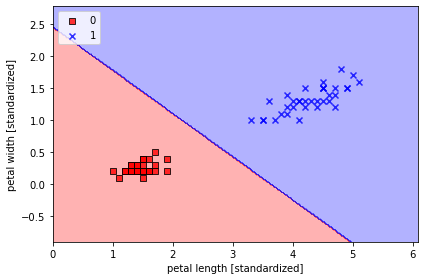
📍 아달린 구현을 로지스틱 회귀 알고리즘으로 변경
class LogisticRegresstionGD(object):
    '''경사 하강법을 사용한 로지스틱 회귀 분류기

    매개변수
    ------------
    eta : float
        학습률 ( 0.0과 1.0 사이 )
    n_iter : int
        훈련 데이터셋 반복 횟수
    random_state : int
        가중치 무작위 초기화를 위한 난수 생성기 시드

    속성
    ------------
    w_ : 1d-array
        학습된 가중치
    cost_ : list
        에폭마다 누적된 로지스틱 비용 함수 값

    '''

    def __init__(self, eta=0.05, n_iter=100, random_state=1):
        self.eta = eta
        self.n_iter = n_iter
        self.random_state = random_state

    def fit(self, x, y):
        '''훈련 데이터 학습

        매개 변수
        --------------
        x : { array-like }, shape : [n_samples, n_features ]
            n_samples개의 샘플과 n_features개의 특성으로 이루어진 훈련 데이터
        y : array-like, shape = [ n_samples ]
            타깃 값

        변환값
        ------------
        self : object

        '''
        rgen = np.random.RandomState(self.random_state)
        self.w_ = rgen.normal(loc=0.0, scale=0.01, size=1 + x.shape[1])
        self.cost_ = []

        for i in range(self.n_iter):
            net_input = self.net_input(x)
            output = self.activation(net_input)
            errors = (y - output)
            self.w_[1:] += self.eta * x.T.dot(errors)
            self.w_[0] += self.eta * errors.sum()

            # 제곱 오차합 대신 로지스틱 비용을 계산
            cost = (-y.dot(np.log(output)) - ((1 - y).dot(np.log(1 - output))))
            self.cost_.append(cost)

        return self

    def net_input(self, x):
        '''최종 입력 계산'''
        return np.dot(x, self.w_[1:]) + self.w_[0]

    def activation(self, z):
        '''로지스틱 시그모이드 활성화 계산'''
        return 1. / (1. + np.exp(-np.clip(z, -250, 250)))

    def predict(self, x):
        '''단위 계산 함수를 사용하여 클래스 레이블을 반환'''
        return np.where(self.net_input(x) >= 0.0, 1, 0)
x_train_01_subset = x_train[(y_train == 0) | (y_train == 1)]
y_train_01_subset = y_train[(y_train == 0) | (y_train == 1)]
lrgd = LogisticRegresstionGD(eta=0.05, n_iter=1000, random_state=1)
lrgd.fit(x_train_01_subset, y_train_01_subset)
plot_decision_regions(x=x_train_01_subset, y=y_train_01_subset, classifier=lrgd)
plt.xlabel('petal length [standardized]')
plt.ylabel('petal width [standardized]')
plt.legend(loc='upper left')
plt.tight_layout()
plt.show()
~~>
📍 사이킷럿을 사용하여 로지스틱 회귀 모델 훈련
- sklearn.linear_model.LogisticRegression의 fit 메서드를 사용하여 표준화 처리된 붓꽃 데이터셋의 클래스 세개를 대상으로 모델 훈련
from sklearn.linear_model import LogisticRegression

lr = LogisticRegression(C=100.0, random_state=1)
lr.fit(x_train_std, y_train)

plot_decision_regions(x_combined_std, y_combined, classifier=lr, test_idx=range(105, 150))
plt.xlabel('petal length [standardized]')
plt.ylabel('petal width [standardized]')
plt.legend(loc='upper left')
plt.tight_layout()
plt.show()

~~>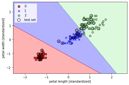
✨ lr = LogisticRegression(C=100.0 ∙∙∙) 에서 C를 통해 규제 강도를 조절
훈련 샘플이 어떤 클래스에 속할 확률은 predict_proba 메서드를 사용하여 계산
lr.predict_proba(x_test_std[:3, :])

~~>
array([[1.52213484e-12, 3.85303417e-04, 9.99614697e-01],
       [9.93560717e-01, 6.43928295e-03, 1.14112016e-15],
[9.98655228e-01, 1.34477208e-03, 1.76178271e-17]])- 첫 번째 행은 첫 번째 붓꽃의 클래스 소속 확률
- 두 번째 행은 두 번째 붗꽃의 클래스 소속 확률
- 열을 모두 더하면 1이 된다
규제를 사용하여 과대적합 피하기
과대적합( overfitting )
- 모델이 훈련 데이터로는 잘 동작하지만 본 적 없는 데이터로는 잘 일반화되지 않는 현상
- 모델이 과대적합일 때 분산이 크다고 말한다
- 모델 파라미터가 너무 많아 주어진 데이터에서 너무 복잡한 모델을 만든 것
과소적합( underfitting )
- 훈련 데이터에 있는 패턴을 감지할 정도로 충분히 모델이 복잡하지 않다는 것을 의미
- 새로운 데이터에서도 성능이 낮다
👉 과대적합, 과소적합을 피하기 위하기 위해서 한가지 방법은 규제를 사용하여 모델의 복잡도를 조정하는 것
- 규제는 공선성( 특성 간의 높은 상관관계 )을 다루거나 데이터에서 잡음을 제거하여 과대적합을 방지할 수 있는 매우 유용한 방법
- 과도한 파라미터 값을 제한하기 위해 추가적인 정보를 주입하는 개념
- 가장 널리 사용하는 규제 형태는 L2 규제이다 ( L2 축소, 가중치 감쇠라고도 부른다 )
- 로지스틱 회귀에서 규제 항을 추가해서 규제를 적용

data science!!, data analyst!! ///// hello world