[10일차]

1. 뉴럴 네트워크 다중분류 실습

• mnist dataset 이용

1) 데이터 준비

• 필요 라이브러리 불러오기

import numpy as np
import pandas as pd
import matplotlib.pyplot as plt
import tensorflow as tf
from tensorflow import keras

# 이미지: 3차원 취급
from keras.datasets import mnist

(X_train, y_train), (X_test, y_test) = mnist.load_data()

print(X_train.shape, y_train.shape)
print(X_test.shape, y_test.shape)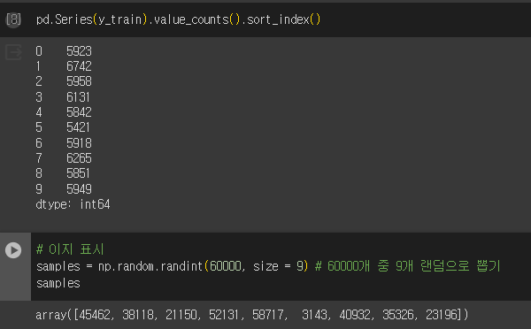

• 이미지 표시

samples = np.random.randint(60000, size = 9) # 60000개 중 9개 랜덤으로 뽑기
plt.figure(figsize=(8,8))

for i, idx in enumerate(samples):
  plt.subplot(3, 3, 1+i) # i가 0부터 시작, matplotlib은 1부터 가리킴
  plt.imshow(X_train[idx], cmap='gray') # 흑백으로
  plt.axis('off') # 축 없애기
  plt.title(y_train[idx])
plt.show()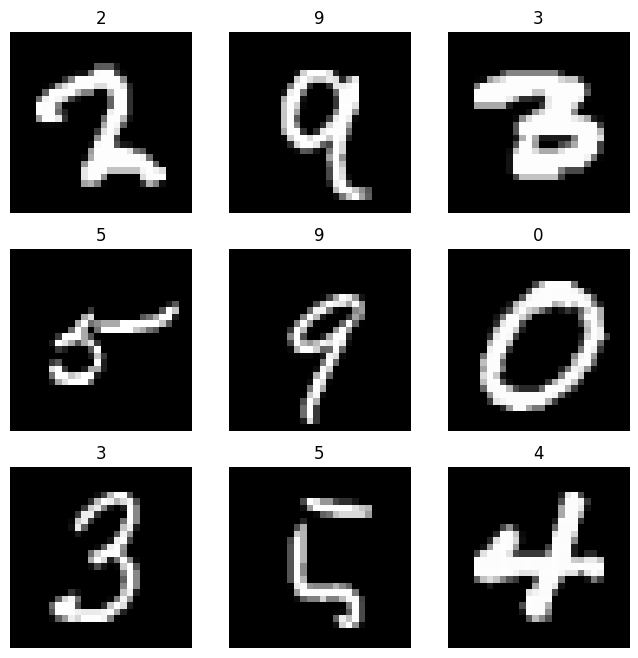

• 검증 데이터 분리

from sklearn.model_selection import train_test_split

X_train, X_val, y_train, y_val = train_test_split(X_train, y_train, test_size=0.2, random_state=42) # 분리

X_train.shape, X_val.shape, y_train.shape, y_val.shape

• 정규화

# 최대.최소 정규화
X_train_s = X_train.astype('float32')/255.
X_val_s = X_val.astype('float32')/255.

np.max(X_train_s), np.min(X_train_s) # 최댓값:1, 최솟값:0 확인

# 레이블값 원핫 인코딩
from keras.utils import to_categorical

y_train_o = to_categorical(y_train)
y_val_o = to_categorical(y_val)

y_train_o[:5] # 확인

# flatten(펼치기)
X_train_s = X_train_s.reshape(-1, 28*28) # -1: 알아서 계산해줘
X_val_s = X_val_s.reshape(-1, 28*28) 

2) 모델 만들기

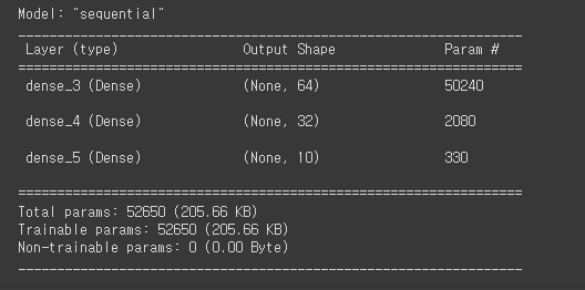
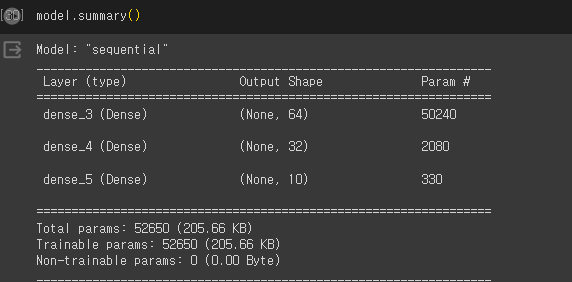
from keras import layers

model = keras.Sequential([
    layers.Dense(units=64, activation='relu', input_shape=(28*28, )),
    layers.Dense(units=32, activation='relu'),
    layers.Dense(units=10, activation='softmax')
                         
])

3) 학습

model.compile(
    optimizer='adam',
    loss='categorical_crossentropy',
    metrics=['accuracy']
)

EPOCHS=10
BATCH_SIZE=64

history = model.fit(
    X_train_s, y_train_o,
    epochs=EPOCHS,
    batch_size = BATCH_SIZE,
     validation_data=(X_val_s, y_val_o),
    verbose=1,
    )

• 그래프

def plot_history(history):
    hist = pd.DataFrame(history.history)
    hist['epoch'] = history.epoch

    plt.figure(figsize=(16, 8))
    plt.subplot(1,2,1)
    plt.xlabel('epoch')
    plt.ylabel('loss')
    plt.plot(hist['epoch'], hist['loss'], label='train loss')
    plt.plot(hist['epoch'], hist['val_loss'], label='val loss')
    plt.legend()

    plt.subplot(1,2,2)
    plt.xlabel('epoch')
    plt.ylabel('accuracy')
    plt.plot(hist['epoch'], hist['accuracy'], label='train accuracy')
    plt.plot(hist['epoch'], hist['val_accuracy'], label='val accuracy')
    plt.legend()
    plt.show()
    
    plot_history(history)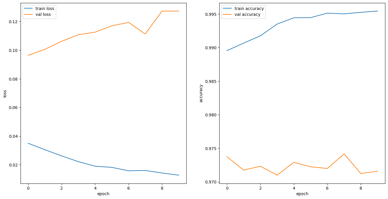

4) 평가

• 테스트 데이터 정리
  : 정규화
  : 차원 변경
  : 레이블 원핫 인코딩

X_test_s = X_test.astype('float32')/255.
X_test_s = X_test_s.reshape(-1, 28*28)

y_test_o = to_categorical(y_test)

5) 예측

y_pred = model.predict(X_test_s)
y_pred = np.argmax(y_pred, axis=1)

# 정확도
from sklearn.metrics import accuracy_score, recall_score, precision_score, f1_score

def print_metrics(y_test, y_pred):
    print(f'accuracy : {accuracy_score(y_test, y_pred) }')
    print(f'recall : {recall_score(y_test, y_pred, average="macro") }')
    print(f'precision : {precision_score(y_test, y_pred, average="macro") }')
    print(f'f1 : {f1_score(y_test, y_pred, average="macro") }')

print_metrics(y_test, y_pred)

• 오답 확인

samples = np.where(y_test != y_pred)[0]
samples = np.random.choice(samples,9)
samples

# 이미지 표시
plt.figure(figsize=(8, 8))
for i, idx in enumerate(samples):
    plt.subplot(3, 3, 1+i)
    plt.imshow(X_test[idx], cmap='gray')
    plt.axis('off')
    plt.title(f'{y_test[idx]}  (pred={y_pred[idx]})')
plt.show()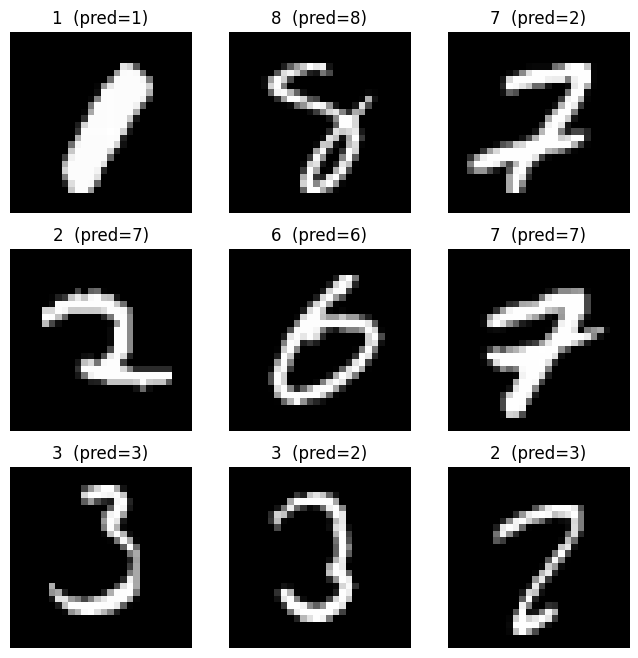

6) 모델 저장

• 케라스 모델로 저장

model.save('nn-mnist-28*28-97.keras') # 정확도; 97 -> 저장된 파일 다운 받아서 백에서 사용

• 텐서플로우 방식

model.save('my_model')

7) 모델 로딩

loaded_model = keras.models.load_model('nn-mnist-28*28-97.keras')